11 MPI topic: Topologies

A communicator describes a group of processes, but the structure of your computation may not be such that every process will communicate with every other process. For instance, in a computation that is mathematically defined on a Cartesian 2D grid, the processes themselves act as if they are two-dimensionally ordered and communicate with N/S/E/W neighbors. If MPI had this knowledge about your application, it could conceivably optimize for it, for instance by renumbering the ranks so that communicating processes are closer together physically in your cluster.

The mechanism to declare this structure of a computation to MPI is known as a virtual topology  . The following types of topology are defined:

• MPI_UNDEFINED : this values holds for communicators where no topology has explicitly been specified.
• MPI_CART : this value holds for Cartesian toppologies, where processes act as if they are ordered in a multi-dimensional `brick'; see section  11.1  .
• MPI_GRAPH : this value describes the graph topology that was defined in MPI-1; section  11.2.4  . It is unnecessarily burdensome, since each process needs to know the total graph, and should therefore be considered obsolete; the type MPI_DIST_GRAPH should be used instead.
• MPI_DIST_GRAPH : this value describes the distributed graph topology where each process only describes the edges in the process graph that touch itself; see section  11.2  .

11.1 Cartesian grid topology

crumb trail: > mpi-topo > Cartesian grid topology

A Cartesian grid is a structure, typically in 2 or 3 dimensions, of points that have two neighbors in each of the dimensions. Thus, if a Cartesian grid has sizes $K\times M\times N$, its points have coordinates $(k,m,n)$ with $0\leq kwraparound connections is called a periodic grid  .

The auxiliary routine MPI_Dims_create assists in finding a grid of a given dimension, attempting to minimize the diameter. { \def\snippetcodefraction{.45} \def\snippetlistfraction{.55} \csnippetwithoutput{dimscreate}{examples/mpi/c}{cartdims} } If the dimensions array is nonzero in a component, that one is not touched. Of course, the product of the specified dimensions has to divide in the input number of nodes.

11.1.1 Cartesian topology communicator

crumb trail: > mpi-topo > Cartesian grid topology > Cartesian topology communicator

The cartesian topology is specified by giving MPI_Cart_create the sizes of the processor grid along each axis, and whether the grid is periodic along that axis.

MPI_Comm cart_comm;
int *periods = (int*) malloc(dim*sizeof(int));
for ( int id=0; id<dim; id++ ) periods[id] = 0;
MPI_Cart_create
  ( comm,dim,dimensions,periods,
    0,&cart_comm );

(The Cartesian grid can have fewer processes than the input communicator: any processes not included get MPI_COMM_NULL as output.)

For a given communicator, you can test what type it is with MPI_Topo_test :

int world_type,cart_type;
MPI_Topo_test( comm,&world_type);
MPI_Topo_test( cart_comm,&cart_type );
if (procno==0) {
  printf("World comm type=%d, Cart comm type=%d\n",
         world_type,cart_type);
  printf("no topo        =%d, cart top      =%d\n",
         MPI_UNDEFINED,MPI_CART);
}

For a Cartesian communicator, you can retrieve its information with MPI_Cartdim_get and MPI_Cart_get :

int dim;
MPI_Cartdim_get( cart_comm,&dim );
int *dimensions = (int*) malloc(dim*sizeof(int));
int *periods    = (int*) malloc(dim*sizeof(int));
int *coords     = (int*) malloc(dim*sizeof(int));
MPI_Cart_get( cart_comm,dim,dimensions,periods,coords );

11.1.2 Cartesian vs world rank

crumb trail: > mpi-topo > Cartesian grid topology > Cartesian vs world rank

Each point in this new communicator has a coordinate and a rank. The translation from rank to Cartesian coordinate is done by MPI_Cart_coords  , and translation from coordinates to a rank is done by MPI_Cart_rank  . In both cases, this translation can be done on any process; for the latter routine note that coordinates outside the Cartesian grid are erroneous, if the grid is not periodic in the offending coordinate.

// cart.c
MPI_Comm comm2d;
int periodic[ndim]; periodic[0] = periodic[1] = 0;
MPI_Cart_create(comm,ndim,dimensions,periodic,1,&comm2d);
MPI_Cart_coords(comm2d,procno,ndim,coord_2d);
MPI_Cart_rank(comm2d,coord_2d,&rank_2d);
printf("I am %d: (%d,%d); originally %d\n",
       rank_2d,coord_2d[0],coord_2d[1],procno);

The reorder parameter to MPI_Cart_create indicates whether processes can have a rank in the new communicator that is different from in the old one.

11.1.3 Cartesian communication

crumb trail: > mpi-topo > Cartesian grid topology > Cartesian communication

A common communication pattern in Cartesian grids is to do an MPI_Sendrecv with processes that are adjacent along one coordinate axis.

By way of example, consider a 3D grid that is periodic in the first dimension:

// cartcoord.c
for ( int id=0; id<dim; id++)
  periods[id] = id==0 ? 1 : 0;
MPI_Cart_create
  ( comm,dim,dimensions,periods,
    0,&period_comm );

We shift process 0 in dimensions 0 and 1. In dimension 0 we get a wrapped-around source, and a target that is the next process in row-major ordering; in dimension 1 we get MPI_PROC_NULL as source, and a legitimate target. \csnippetwithoutput{cartshift01}{examples/mpi/c}{cartshift}

11.1.4 Communicators in subgrids

crumb trail: > mpi-topo > Cartesian grid topology > Communicators in subgrids

The routine MPI_Cart_sub is similar to MPI_Comm_split  , in that it splits a communicator into disjoint subcommunicators. In this case, it splits a Cartesian communicator into disjoint Cartesian communicators, each corresponding to a subset of the dimensions. This subset inherits both sizes and periodicity from the original communicator.

\csnippetwithoutput{hyperplane13p}{examples/mpi/c}{cartsub}

11.1.5 Reordering

crumb trail: > mpi-topo > Cartesian grid topology > Reordering

The MPI_Cart_create routine has a possibility of reordering ranks. If this is applied, the routine MPI_Cart_map gives the result of this. Given the same parameters as MPI_Cart_create  , it returns the re-ordered rank for the calling process.

11.2 Distributed graph topology

crumb trail: > mpi-topo > Distributed graph topology

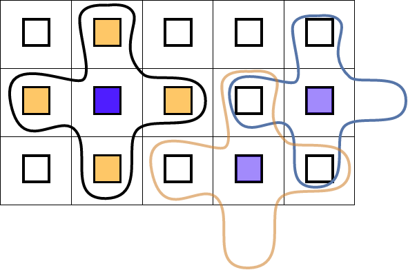\caption{Illustration of a distributed graph topology where each node has four neighbors}

In many calculations on a grid (using the term in its mathematical, FEM  , sense), a grid point will collect information from grid points around it. Under a sensible distribution of the grid over processes, this means that each process will collect information from a number of neighbor processes. The number of neighbors is dependent on that process. For instance, in a 2D grid (and assuming a five-point stencil for the computation) most processes communicate with four neighbors; processes on the edge with three, and processes in the corners with two.

Such a topology is illustrated in figure  11.2  .

MPI's notion of \indextermbusdef{graph}{topology}, and the neighborhood collectives  , offer an elegant way of expressing such communication structures. There are various reasons for using graph topologies over the older, simpler methods.

• MPI is allowed to reorder the processes, so that network proximity in the cluster corresponds to proximity in the structure of the code.
• Ordinary collectives could not directly be used for graph problems, unless one would adopt a subcommunicator for each graph neighborhood. However, scheduling would then lead to deadlock or serialization.
• The normal way of dealing with graph problems is through nonblocking communications. However, since the user indicates an explicit order in which they are posted, congestion at certain processes may occur.
• Collectives can pipeline data, while send/receive operations need to transfer their data in its entirety.
• Collectives can use spanning trees, while send/receive uses a direct connection.

Thus the minimal description of a process graph contains for each process:

• Degree: the number of neighbor processes; and
• the ranks of the processes to communicate with.

• MPI_Dist_graph_create_adjacent assumes that a process knows both who it is sending it, and who will send to it. This is the most work for the programmer to specify, but it is ultimately the most efficient.
• MPI_Dist_graph_create specifies on each process only what it is the source for; that is, who this process will be sending to. Consequently, some amount of processing -- including communication -- is needed to build the converse information, the ranks that will be sending to a process.

11.2.1 Graph creation

crumb trail: > mpi-topo > Distributed graph topology > Graph creation

There are two creation routines for process graphs. These routines are fairly general in that they allow any process to specify any part of the topology. In practice, of course, you will mostly let each process describe its own neighbor structure.

The routine MPI_Dist_graph_create_adjacent assumes that a process knows both who it is sending it, and who will send to it. This means that every edge in the communication graph is represented twice, so the memory footprint is double of what is strictly necessary. However, no communication is needed to build the graph.

The second creation routine, MPI_Dist_graph_create  , is probably easier to use, especially in cases where the communication structure of your program is symmetric, meaning that a process sends to the same neighbors that it receives from. Now you specify on each process only what it is the source for; that is, who this process will be sending to.\footnote{I disagree with this design decision. Specifying your sources is usually easier than specifying your destinations.}. Consequently, some amount of processing -- including communication -- is needed to build the converse information, the ranks that will be sending to a process.

MPL note The class mpl:: dist_graph_communicator only has a constructor corresponding to MPI_Dist_graph_create  . End of MPL note

Figure  11.2 describes the common five-point stencil structure. If we let each process only describe itself, we get the following:

• nsources $=1$ because the calling process describes on node in the graph: itself.
• sources is an array of length 1, containing the rank of the calling process.
• degrees is an array of length 1, containing the degree (probably: 4) of this process.
• destinations is an array of length the degree of this process, probably again 4. The elements of this array are the ranks of the neighbor nodes; strictly speaking the ones that this process will send to.
• weights is an array declaring the relative importance of the destinations. For an unweighted graph use MPI_UNWEIGHTED  . In the case the graph is weighted, but the degree of a source is zero, you can pass an empty array as MPI_WEIGHTS_EMPTY  .
• reorder ( int in C, LOGICAL in Fortran) indicates whether MPI is allowed to shuffle processes to achieve greater locality.

The resulting communicator has all the processes of the original communicator, with the same ranks. In other words MPI_Comm_size and MPI_Comm_rank gives the same values on the graph communicator, as on the intra-communicator that it is constructed from. To get information about the grouping, use MPI_Dist_graph_neighbors and MPI_Dist_graph_neighbors_count ; section  11.2.3  .

By way of example we build an unsymmetric graph, that is, an edge $v_1\rightarrow v_2$ between vertices $v_1,v_2$ does not imply an edge $v_2\rightarrow v_1$.

Here we gather the coordinates of the source neighbors:

{ \def\snippetcodefraction{.45} \def\snippetlistfraction{.5} \csnippetwithoutput{distgraphreadout}{examples/mpi/c}{graph} }

However, we can't rely on the sources being ordered, so the following segment performs an explicit query for the source neighbors:

{ \def\snippetcodefraction{.45} \def\snippetlistfraction{.5} \csnippetwithoutput{distgraphcount}{examples/mpi/c}{graphcount} }

Python note Graph communicator creation is a method of the \plstinline{Comm} class, and the graph communicator is a function return result:

graph_comm = oldcomm.Create_dist_graph(sources, degrees, destinations)

MPL note The constructor dist_graph_communicator

dist_graph_communicator
   (const communicator &old_comm, const source_set &ss,
    const dest_set &ds, bool reorder = true);    

11.2.2 Neighbor collectives

crumb trail: > mpi-topo > Distributed graph topology > Neighbor collectives

We can now use the graph topology to perform a gather or allgather MPI_Neighbor_allgather that combines only the processes directly connected to the calling process.

The neighbor collectives have the same argument list as the regular collectives, but they apply to a graph communicator.

\caption{Solving the right-send exercise with neighborhood collectives}

Exercise Revisit exercise  4.1.4.3 and solve it using MPI_Dist_graph_create  . Use figure  11.2.2 for inspiration.

Use a degree value of 1. (There is a skeleton code rightgraph in the repository)
End of exercise

The previous exercise can be done with a degree value of:

• 1, reflecting that each process communicates with just 1 other; or
• 2, reflecting that you really gather from two processes.

Another neighbor collective is MPI_Neighbor_alltoall  .

The vector variants are MPI_Neighbor_allgatherv and MPI_Neighbor_alltoallv  .

There is a heterogenous (multiple datatypes) variant: MPI_Neighbor_alltoallw  .

The list is: MPI_Neighbor_allgather  , MPI_Neighbor_allgatherv  , MPI_Neighbor_alltoall  , MPI_Neighbor_alltoallv  , MPI_Neighbor_alltoallw  .

Nonblocking: MPI_Ineighbor_allgather  , MPI_Ineighbor_allgatherv  , MPI_Ineighbor_alltoall  , MPI_Ineighbor_alltoallv  , MPI_Ineighbor_alltoallw  .

For unclear reasons there is no MPI_Neighbor_allreduce  .

11.2.3 Query

crumb trail: > mpi-topo > Distributed graph topology > Query

There are two routines for querying the neighbors of a process: MPI_Dist_graph_neighbors_count and MPI_Dist_graph_neighbors  .

While this information seems derivable from the graph construction, that is not entirely true for two reasons.

1. With the nonadjoint version MPI_Dist_graph_create  , only outdegrees and destinations are specified; this call then supplies the indegrees and sources;
2. As observed above, the order in which data is placed in the receive buffer of a gather call is not determined by the create call, but can only be queried this way.

11.2.4 Graph topology (deprecated)

crumb trail: > mpi-topo > Distributed graph topology > Graph topology (deprecated)

The original MPI-1 had a graph topology interface MPI_Graph_create which required each process to specify the full process graph. Since this is not scalable, it should be considered deprecated. Use the distributed graph topology (section  11.2  ) instead.

Other legacy routines: MPI_Graph_neighbors  , MPI_Graph_neighbors_count  , MPI_Graph_get  , MPI_Graphdims_get  .

11.2.5 Re-ordering

crumb trail: > mpi-topo > Distributed graph topology > Re-ordering

Similar to the MPI_Cart_map routine (section  11.1.5  ), the routine MPI_Graph_map gives a re-ordered rank for the calling process.