\[ % mathjax inclusion. \newcommand\bbP{\mathbb{P}} \newcommand\bbR{\mathbb{R}} \newcommand\becomes{\mathop{:=}} \newcommand\dtdxx{\frac{\alpha\Delta t}{\Delta x^2}} \newcommand\defined{ \mathrel{\lower 5pt \hbox{${\equiv\atop\mathrm{\scriptstyle D}}$}}} \newcommand\fp[2]{#1\cdot10^{#2}} \newcommand\inv{^{-1}}\newcommand\invt{^{-t}} \newcommand\macro[1]{$\langle$#1$\rangle$} \newcommand\nobreak{} \newcommand\Rn{{\cal R}^n} \newcommand\Rnxn{{\cal R}^{n\times x}} \newcommand\sublocal{_{\mathrm\scriptstyle local}} \newcommand\toprule{\hline} \newcommand\midrule{\hline} \newcommand\bottomrule{\hline} \newcommand\multicolumn[3]{#3} \newcommand\defcolvector[2]{\begin{pmatrix} #1_0

#1_1


vdots

#1_{#2-1} \end{pmatrix}} % {
left(
begin{array}{c} #1_0

#1_1


vdots

#1_{#2-1}
end{array}
right) } \] 2.1 : Introduction
2.1.1 : Functional parallelism versus data parallelism
2.1.2 : Parallelism in the algorithm versus in the code
2.2 : Theoretical concepts
2.2.1 : Definitions
2.2.1.1 : Speedup and efficiency
2.2.1.2 : Cost-optimality
2.2.2 : Asymptotics
2.2.3 : Amdahl's law
2.2.3.1 : Amdahl's law with communication overhead
2.2.3.2 : Gustafson's law
2.2.3.3 : Amdahl's law and hybrid programming
2.2.4 : Critical path and Brent's theorem
2.2.5 : Scalability
2.2.5.1 : Iso-efficiency
2.2.5.2 : Precisely what do you mean by scalable?
2.2.6 : Simulation scaling
2.2.7 : Other scaling measures
2.2.8 : Concurrency; asynchronous and distributed computing
2.3 : Parallel Computers Architectures
2.3.1 : SIMD
2.3.1.1 : Pipelining and pipeline processors
2.3.1.2 : True SIMD in CPUs and GPUs
2.3.2 : MIMD / SPMD computers
2.3.3 : The commoditization of supercomputers
2.4 : Different types of memory access
2.4.1 : Symmetric Multi-Processors: Uniform Memory Access
2.4.2 : Non-Uniform Memory Access
2.4.2.1 : Affinity
2.4.2.2 : Coherence
2.4.3 : Logically and physically distributed memory
2.5 : Granularity of parallelism
2.5.1 : Data parallelism
2.5.2 : Instruction-level parallelism
2.5.3 : Task-level parallelism
2.5.4 : Conveniently parallel computing
2.5.5 : Medium-grain data parallelism
2.5.6 : Task granularity
2.6 : Parallel programming
2.6.1 : Thread parallelism
2.6.1.1 : The fork-join mechanism
2.6.1.2 : Hardware support for threads
2.6.1.3 : Threads example
2.6.1.4 : Contexts
2.6.1.5 : Race conditions, thread safety, and atomic operations
2.6.1.6 : Memory models and sequential consistency
2.6.1.7 : Affinity
2.6.1.8 : Cilk Plus
2.6.1.9 : Hyperthreading versus multi-threading
2.6.2 : OpenMP
2.6.2.1 : OpenMP examples
2.6.3 : Distributed memory programming through message passing
2.6.3.1 : The global versus the local view in distributed programming
2.6.3.2 : Blocking and non-blocking communication
2.6.3.3 : The MPI library
2.6.3.4 : Blocking
2.6.3.5 : Collective operations
2.6.3.6 : Non-blocking communication
2.6.3.7 : MPI version 1 and 2 and 3
2.6.3.8 : One-sided communication
2.6.4 : Hybrid shared/distributed memory computing
2.6.5 : Parallel languages
2.6.5.1 : Discussion
2.6.5.2 : Unified Parallel C
2.6.5.3 : High Performance Fortran
2.6.5.4 : Co-array Fortran
2.6.5.5 : Chapel
2.6.5.6 : Fortress
2.6.5.7 : X10
2.6.5.8 : Linda
2.6.5.9 : The Global Arrays library
2.6.6 : OS-based approaches
2.6.7 : Active messages
2.6.8 : Bulk synchronous parallelism
2.6.9 : Data dependencies
2.6.9.1 : Types of data dependencies
2.6.9.2 : Parallelizing nested loops
2.6.10 : Program design for parallelism
2.6.10.1 : Parallel data structures
2.6.10.2 : Latency hiding
2.7 : Topologies
2.7.1 : Some graph theory
2.7.2 : Busses
2.7.3 : Linear arrays and rings
2.7.4 : 2D and 3D arrays
2.7.5 : Hypercubes
2.7.5.1 : Embedding grids in a hypercube
2.7.6 : Switched networks
2.7.6.1 : Cross bar
2.7.6.2 : Butterfly exchange
2.7.6.3 : Fat-trees
2.7.6.4 : Over-subscription and contention
2.7.7 : Cluster networks
2.7.7.1 : Case study: Stampede
2.7.7.2 : Case study: Cray Dragonfly networks
2.7.8 : Bandwidth and latency
2.7.9 : Locality in parallel computing
2.8 : Multi-threaded architectures
2.9 : Co-processors, including GPUs
2.9.1 : A little history
2.9.2 : Bottlenecks
2.9.3 : GPU computing
2.9.3.1 : SIMD-type programming with kernels
2.9.3.2 : GPUs versus CPUs
2.9.3.3 : Expected benefit from GPUs
2.9.4 : Intel Xeon Phi
2.10 : Load balancing
2.10.1 : Load balancing versus data distribution
2.10.2 : Load scheduling
2.10.3 : Load balancing of independent tasks
2.10.4 : Load balancing as graph problem
2.10.5 : Load redistributing
2.10.5.1 : Diffusion load balancing
2.10.5.2 : Load balancing with space-filling curves
2.11 : Remaining topics
2.11.1 : Distributed computing, grid computing, cloud computing
2.11.2 : Usage scenarios
2.11.3 : Characterization
2.11.4 : Capability versus capacity computing
2.11.5 : MapReduce
2.11.5.1 : Expressive power of the MapReduce model
2.11.5.2 : Mapreduce software
2.11.5.3 : Implementation issues
2.11.5.4 : Functional programming
2.11.6 : The top500 list
2.11.6.1 : The top500 list as a recent history of supercomputing
2.11.7 : Heterogeneous computing
Back to Table of Contents

2 Parallel Computing

The largest and most powerful computers are sometimes called `supercomputers'. For the last two decades, this has, without exception, referred to parallel computers: machines with more than one CPU that can be set to work on the same problem.

Parallelism is hard to define precisely, since it can appear on several levels. In the previous chapter you already saw how inside a CPU several instructions can be `in flight' simultaneously. This is called instruction-level parallelism  , and it is outside explicit user control: it derives from the compiler and the CPU deciding which instructions, out of a single instruction stream, can be processed simultaneously. At the other extreme is the sort of parallelism where more than one instruction stream is handled by multiple processors, often each on their own circuit board. This type of parallelism is typically explicitly scheduled by the user.

In this chapter, we will analyze this more explicit type of parallelism, the hardware that supports it, the programming that enables it, and the concepts that analyze it.

2.1 Introduction

crumb trail: > parallel > Introduction

In scientific codes, there is often a large amount of work to be done, and it is often regular to some extent, with the same operation being performed on many data. The question is then whether this work can be sped up by use of a parallel computer. If there are $n$ operations to be done, and they would take time $t$ on a single processor, can they be done in time $t/p$ on $p$ processors?

Let us start with a very simple example. Adding two vectors of length $n$

for (i=0; i<n; i++)
  a[i] = b[i] + c[i];

can be done with up to $n$ processors. In the idealized case with $n$ processors, each processor has local scalars a,b,c and executes

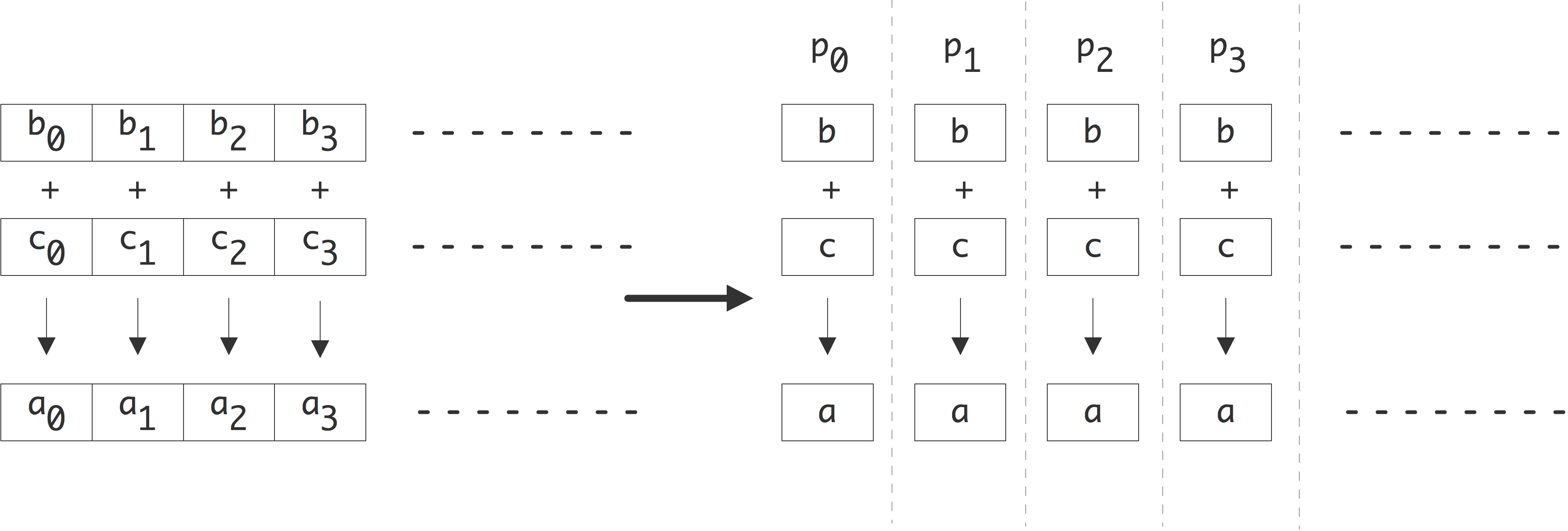
FIGURE 2.1: Parallelization of a vector addition.

the single instruction a=b+c  . This is depicted in figure  2.1  .

In the general case, where each processor executes something like

for (i=my_low; i<my_high; i++)
  a[i] = b[i] + c[i];

execution time is linearly reduced with the number of processors. If each operation takes a unit time, the original algorithm takes time $n$, and the parallel execution on $p$ processors $n/p$. The parallel algorithm is faster by a factor of $p$%

(Note: {Here we ignore lower order errors in this result when $p$ does not divide perfectly in $n$. We will also, in general, ignore matters of loop overhead.}  )

 .

Next, let us consider summing the elements of a vector. (An operation that has a vector as input but only a scalar as output is often called a reduction  .) We again assume that each processor contains just a single array element. The sequential code:

s = 0;
for (i=0; i<n; i++)
  s += x[i]

is no longer obviously parallel, but if we recode the loop as

for (s=2; s<2*n; s*=2)
  for (i=0; i<n-s/2; i+=s)
    x[i] += x[i+s/2]

there is a way to parallelize it: every iteration of the outer loop is now a loop that can be done by $n/s$ processors in parallel. Since the

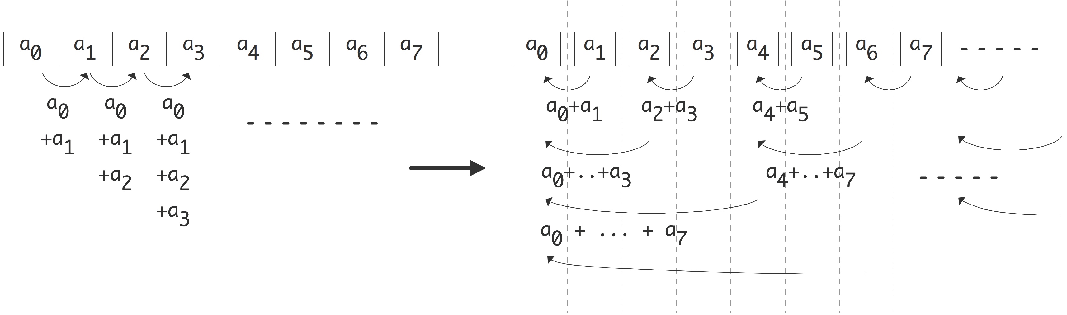
FIGURE 2.2: Parallelization of a vector reduction.

outer loop will go through $\log_2n$ iterations, we see that the new algorithm has a reduced runtime of $n/p\cdot\log_2 n$. The parallel algorithm is now faster by a factor of $p/\log_2n$. This is depicted in figure  2.2  .

Even from these two simple examples we can see some of the characteristics of parallel computing:

• Sometimes algorithms need to be rewritten slightly to make them parallel.
• A parallel algorithm may not show perfect speedup.

There are other things to remark on. In the first case, if each processors has its $x_i,y_i$ in a local store the algorithm can be executed without further complications. In the second case, processors need to communicate data among each other and we haven't assigned a cost to that yet.

First let us look systematically at communication. We can take the parallel algorithm in the right half of figure  2.2 and turn it into a tree graph (see Appendix  app:graph  ) by defining the inputs as leave nodes, all partial sums as interior nodes, and the root as the total sum. There is an edge from one node to another if the first is input to the (partial) sum in the other. This is illustrated in figure  2.3  . In this figure nodes are horizontally aligned with other computations that can be performed simultaneously; each level is sometimes called a superstep in the computation. Nodes are vertically aligned if they are computed on the same processors, and an arrow corresponds to a communication if it goes from one processor to another.

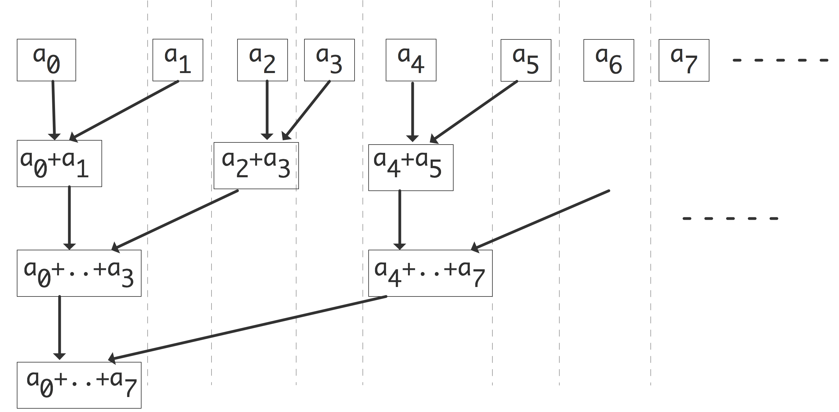
FIGURE 2.3: Communication structure of a parallel vector reduction.

The vertical alignment in figure  2.3 is not the only one possible. If nodes are shuffled within a superstep or horizontal level, a different communication pattern arises.

Exercise Consider placing the nodes within a superstep on random processors. Show that, if no two nodes wind up on the same processor, at most twice the number of communications is performed from the case in figure  2.3  .
End of exercise

Exercise Can you draw the graph of a computation that leaves the sum result on each processor? There is a solution that takes twice the number of supersteps, and there is one that takes the same number. In both cases the graph is no longer a tree, but a more general DAG  .
End of exercise

Processors are often connected through a network, and moving data through this network takes time. This introduces a concept of distance between the processors. In figure  2.3  , where the processors are linearly ordered, this is related to their rank in the ordering. If the network only connects a processor with its immediate neighbors, each iteration of the outer loop increases the distance over which communication takes place.

Exercise Assume that an addition takes a certain unit time, and that moving a number from one processor to another takes that same unit time. Show that the communication time equals the computation time.

Now assume that sending a number from processor $p$ to $p\pm k$ takes time $k$. Show that the execution time of the parallel algorithm now is of the same order as the sequential time.
End of exercise

The summing example made the unrealistic assumption that every processor initially stored just one vector element: in practice we will have $p

Exercise Consider the case of summing 8 elements with 4 processors. Show that some of the edges in the graph of figure  2.3 no longer correspond to actual communications. Now consider summing 16 elements with, again, 4 processors. What is the number of communication edges this time?
End of exercise

These matters of algorithm adaptation, efficiency, and communication, are crucial to all of parallel computing. We will return to these issues in various guises throughout this chapter.

2.1.1 Functional parallelism versus data parallelism

crumb trail: > parallel > Introduction > Functional parallelism versus data parallelism

From the above introduction we can describe parallelism as finding independent operations in the execution of a program. In all of the examples these independent operations were in fact identical operations, but applied to different data items. We could call this data parallelism : the same operation is applied in parallel to many data elements. This is in fact a common scenario in scientific computing: parallelism often stems from the fact that a data set (vector, matrix, graph,\ldots) is spread over many processors, each working on its part of the data.

The term data parallelism is traditionally mostly applied if the operation is a single instruction; in the case of a subprogram it is often called task parallelism  .

It is also possible to find independence, not based on data elements, but based on the instructions themselves. Traditionally, compilers analyze code in terms of ILP : independent instructions can be given to separate floating point units, or reordered, for instance to optimize register usage (see also section  2.5.2  ). ILP is one case of functional parallelism ; on a higher level, functional parallelism can be obtained by considering independent subprograms, often called task parallelism ; see section  2.5.3  .

Some examples of functional parallelism are Monte Carlo simulations, and other algorithms that traverse a parametrized search space, such as boolean satisfyability problems.

2.1.2 Parallelism in the algorithm versus in the code

crumb trail: > parallel > Introduction > Parallelism in the algorithm versus in the code

Often we are in the situation that we want to parallelize an algorithm that has a common expression in sequential form. In some cases, this sequential form is straightforward to parallelize, such as in the vector addition discussed above. In other cases there is no simple way to parallelize the algorithm; we will discuss linear recurrences in section  6.9.2  . And in yet another case the sequential code may look not parallel, but the algorithm actually has parallelism.

Exercise

for i in [1:N]:
    x[0,i] = some_function_of(i)
    x[i,0] = some_function_of(i)

for i in [1:N]:
    for j in [1:N]:
        x[i,j] = x[i-1,j]+x[i,j-1]

Answer the following questions about the double i,j loop:

1. Are the iterations of the inner loop independent, that is, could they be executed simultaneously?
2. Are the iterations of the outer loop independent?
3. If x[1,1] is known, show that x[2,1] and x[1,2] can be computed independently.
4. Does this give you an idea for a parallelization strategy?

End of exercise

We will discuss the solution to this conundrum in section  6.9.1  . In general, the whole of chapter  High performance linear algebra will be about the amount of parallelism intrinsic in scientific computing algorithms.

2.2 Theoretical concepts

crumb trail: > parallel > Theoretical concepts

There are two important reasons for using a parallel computer: to have access to more memory or to obtain higher performance. It is easy to characterize the gain in memory, as the total memory is the sum of the individual memories. The speed of a parallel computer is harder to characterize. This section will have an extended discussion on theoretical measures for expressing and judging the gain in execution speed from going to a parallel architecture.

2.2.1 Definitions

crumb trail: > parallel > Theoretical concepts > Definitions

2.2.1.1 Speedup and efficiency

crumb trail: > parallel > Theoretical concepts > Definitions > Speedup and efficiency

A simple approach to defining speedup is to let the same program run on a single processor, and on a parallel machine with $p$ processors, and to compare runtimes. With $T_1$ the execution time on a single processor and $T_p$ the time on $p$ processors, we define the speedup as $S_p=T_1/T_p$. (Sometimes $T_1$ is defined as `the best time to solve the problem on a single processor', which allows for using a different algorithm on a single processor than in parallel.) In the ideal case, $T_p=T_1/p$, but in practice we don't expect to attain that, so $S_p\leq p$. To measure how far we are from the ideal speedup, we introduce the efficiency $E_p=S_p/p$. Clearly, $0< E_p\leq 1$.

There is a practical problem with the above definitions: a problem that can be solved on a parallel machine may be too large to fit on any single processor. Conversely, distributing a single processor problem over many processors may give a distorted picture since very little data will wind up on each processor. Below we will discuss more realistic measures of speed-up.

There are various reasons why the actual speed is less than $p$. For one, using more than one processor necessitates communication and synchronization, which is overhead that was not part of the original computation. Secondly, if the processors do not have exactly the same amount of work to do, they may be idle part of the time (this is known as load unbalance  ), again lowering the actually attained speedup. Finally, code may have sections that are inherently sequential.

Communication between processors is an important source of a loss of efficiency. Clearly, a problem that can be solved without communication will be very efficient. Such problems, in effect consisting of a number of completely independent calculations, is called embarrassingly parallel (or conveniently parallel ; see section  2.5.4  ); it will have close to a perfect speedup and efficiency.

Exercise The case of speedup larger than the number of processors is called superlinear speedup  . Give a theoretical argument why this can never happen.
End of exercise

In practice, superlinear speedup can happen. For instance, suppose a problem is too large to fit in memory, and a single processor can only solve it by swapping data to disc. If the same problem fits in the memory of two processors, the speedup may well be larger than $2$ since disc swapping no longer occurs. Having less, or more localized, data may also improve the cache behavior of a code.

A form of superlinear speedup can also happen in search algorithms. Imagine that each processor starts in a different location of the search space; now it can happen that, say, processor 3 immediately finds the solution. Sequentially, all the possibilities for processors 1 and 2 would have had to be traversed. The speedup is much greater than 3 in this case.

2.2.1.2 Cost-optimality

crumb trail: > parallel > Theoretical concepts > Definitions > Cost-optimality

In cases where the speedup is not perfect we can define overhead as the difference \begin{equation} T_o = pT_p-T1. \end{equation} We can also interpret this as the difference between simulating the parallel algorithm on a single processor, and the actual best sequential algorithm.

We will later see two different types of overhead:

1. The parallel algorithm can be essentially different from the sequential one. For instance, sorting algorithms have a complexity $O(n\log n)$, but the parallel bitonic sort (section  8.6  ) has complexity $O(n\log^2n)$.
2. The parallel algorithm can have overhead derived from the process or parallelizing, such as the cost of sending messages. As an example, section  6.2.3 analyzes the communication overhead in the matrix-vector product.

A parallel algorithm is called cost-optimal if the overhead is at most of the order of the running time of the sequential algorithm.

Exercise The definition of overhead above implicitly assumes that overhead is not parallelizable. Discuss this assumption in the context of the two examples above.
End of exercise

2.2.2 Asymptotics

crumb trail: > parallel > Theoretical concepts > Asymptotics

If we ignore limitations such as that the number of processors has to be finite, or the physicalities of the interconnect between them, we can derive theoretical results on the limits of parallel computing. This section will give a brief introduction to such results, and discuss their connection to real life high performance computing.

Consider for instance the matrix-matrix multiplication $C=AB$, which takes $2N^3$ operations where $N$ is the matrix size. Since there are no dependencies between the operations for the elements of $C$, we can perform them all in parallel. If we had $N^2$ processors, we could assign each to an $(i,j)$ coordinate in $C$, and have it compute $c_{ij}$ in $2N$ time. Thus, this parallel operation has efficiency $1$, which is optimal.

Exercise Show that this algorithm ignores some serious issues about memory usage:

• If the matrix is kept in shared memory, how many simultaneous reads from each memory locations are performed?
• If the processors keep the input and output to the local computations in local storage, how much duplication is there of the matrix elements?

End of exercise

Adding $N$ numbers $\{x_i\}_{i=1\ldots N}$ can be performed in $\log_2 N$ time with $N/2$ processors. If we have $n/2$ processors we could compute:

1. Define $s^{(0)}_i = x_i$.
2. Iterate with $j=1,\ldots,\log_2 n$:
3. Compute $n/2^j$ partial sums $s^{(j)}_i=s^{(j-1)}_{2i}+s^{(j-1)}_{2i+1}$

We see that the $n/2$ processors perform a total of $n$ operations (as they should) in $\log_2n$ time. The efficiency of this parallel scheme is $O(1/\log_2n)$, a slowly decreasing function of $n$.

Exercise Show that, with the scheme for parallel addition just outlined, you can multiply two matrices in $\log_2 N$ time with $N^3/2$ processors. What is the resulting efficiency?
End of exercise

It is now a legitimate theoretical question to ask

• If we had infinitely many processors, what is the lowest possible time complexity for matrix-matrix multiplication, or
• Are there faster algorithms that still have $O(1)$ efficiency?

Such questions have been researched (see for instance  [He:surveyparallel]  ), but they have little bearing on high performance computing.

A first objection to these kinds of theoretical bounds is that they implicitly assume some form of shared memory. In fact, the formal model for these algorithms is called a PRAM  , where the assumption is that every memory location is accessible to any processor.

Often an additional assumption is made that multiple simultaneous accesses to the same location are in fact possible. Since write and write accesses have a different behavior in practice, there is the concept of CREW-PRAM, for Concurrent Read, Exclusive Write PRAM.

The basic assumptions of the PRAM model are unrealistic in practice, especially in the context of scaling up the problem size and the number of processors. A further objection to the PRAM model is that even on a single processor it ignores the memory hierarchy; section  1.3  .

But even if we take distributed memory into account, theoretical results can still be unrealistic. The above summation algorithm can indeed work unchanged in distributed memory, except that we have to worry about the distance between active processors increasing as we iterate further. If the processors are connected by a linear array, the number of `hops' between active processors doubles, and with that, asymptotically, the computation time of the iteration. The total execution time then becomes $n/2$, a disappointing result given that we throw so many processors at the problem.

What if the processors are connected with a hypercube topology (section  2.7.5  )? It is not hard to see that the summation algorithm can then indeed work in $\log_2n$ time. However, as $n\rightarrow\infty$, can we physically construct a sequence of hypercubes of $n$ nodes and keep the communication time between two connected constant? Since communication time depends on latency, which partly depends on the length of the wires, we have to worry about the physical distance between nearest neighbors.

The crucial question here is whether the hypercube (an $n$-dimensional object) can be embedded in 3-dimensional space, while keeping the distance (measured in meters) constant between connected neighbors. It is easy to see that a 3-dimensional grid can be scaled up arbitrarily while maintaining a unit wire length, but the question is not clear for a hypercube. There, the length of the wires may have to increase as $n$ grows, which runs afoul of the finite speed of electrons.

We sketch a proof (see  [Fisher:fastparallel] for more details) that, in our three dimensional world and with a finite speed of light, speedup is limited to $\sqrt[4]{n}$ for a problem on $n$ processors, no matter the interconnect. The argument goes as follows. Consider an operation that involves collecting a final result on one processor. Assume that each processor takes a unit volume of space, produces one result per unit time, and can send one data item per unit time. Then, in an amount of time $t$, at most the processors in a ball with radius $t$, that is, $O(t^3)$ processors total, can contribute to the final result; all others are too far away. In time $T$, then, the number of operations that can contribute to the final result is $\int_0^T t^3dt=O(T^4)$. This means that the maximum achievable speedup is the fourth root of the sequential time.

Finally, the question `what if we had infinitely many processors' is not realistic as such, but we will allow it in the sense that we will ask the weak scaling question (section  2.2.5  ) `what if we let the problem size and the number of processors grow proportional to each other'. This question is legitimate, since it corresponds to the very practical deliberation whether buying more processors will allow one to run larger problems, and if so, with what `bang for the buck'.

2.2.3 Amdahl's law

crumb trail: > parallel > Theoretical concepts > Amdahl's law

One reason for less than perfect speedup is that parts of a code can be inherently sequential. This limits the parallel efficiency as follows. Suppose that $5\%$ of a code is sequential, then the time for that part can not be reduced, no matter how many processors are available. Thus, the speedup on that code is limited to a factor Law}  [amd:law]  , which we will now formulate.

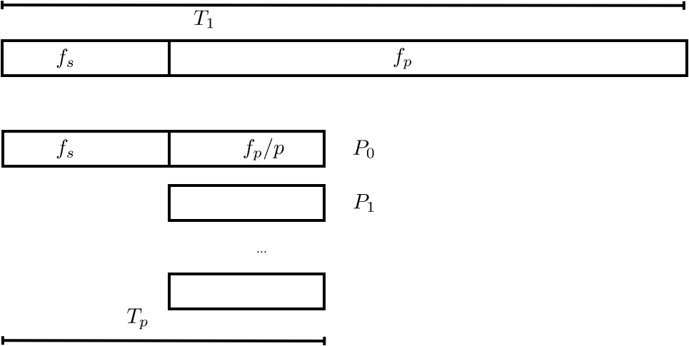
FIGURE 2.4: Sequential and parallel time in Amdahl's analysis.

Let $F_s$ be the sequential fraction and $F_p$ be the parallel fraction (or more strictly: the `parallelizable' fraction) of a code, respectively. Then $F_p+F_s=1$. The parallel execution time $T_p$ on $p$ processors is the sum of the part that is sequential $T_1F_s$ and the part that can be parallelized $T_1F_p/P$: \begin{equation} T_P=T_1(F_s+F_p/P). \label{eq:amdahl} \end{equation} (see figure  2.4  ) As the number of processors grows $P\rightarrow\infty$, the parallel execution time now approaches that of the sequential fraction of the code: $T_P\downarrow T_1F_s$. We conclude that speedup is limited by $S_P\leq 1/F_s$ and efficiency is a decreasing function $E\sim 1/P$.

The sequential fraction of a code can consist of things such as I/O operations. However, there are also parts of a code that in effect act as sequential. Consider a program that executes a single loop, where all iterations can be computed independently. Clearly, this code offers no obstacles to parallelization. However by splitting the loop in a number of parts, one per processor, each processor now has to deal with loop overhead: calculation of bounds, and the test for completion. This overhead is replicated as many times as there are processors. In effect, loop overhead acts as a sequential part of the code.

Exercise Let's do a specific example. Assume that a code has a setup that takes 1 second and a parallelizable section that takes 1000 seconds on one processor. What are the speedup and efficiency if the code is executed with 100 processors? What are they for 500 processors? Express your answer to at most two significant digits.
End of exercise

Exercise Investigate the implications of Amdahl's law: if the number of processors $P$ increases, how does the parallel fraction of a code have to increase to maintain a fixed efficiency?
End of exercise

2.2.3.1 Amdahl's law with communication overhead

crumb trail: > parallel > Theoretical concepts > Amdahl's law > Amdahl's law with communication overhead

In a way, Amdahl's law, sobering as it is, is even optimistic. Parallelizing a code will give a certain speedup, but it also introduces communication overhead that will lower the speedup attained. Let us refine our model of 2.4 \cite[p. 367]{Landau:comp-phys}): \begin{equation} T_p= T_1(F_s+F_p/P) +T_c, \end{equation} where $T_c$ is a fixed communication time.

To assess the influence of this communication overhead, we assume that the code is fully parallelizable, that is, $F_p=1$. We then find that \begin{equation} S_p=\frac{T_1}{T_1/p+T_c}. \label{eq:amdahl-comm} \end{equation} For this to be close to $p$, we need $T_c\ll T_1/p$ or $p\ll T_1/T_c$. In other words, the number of processors should not grow beyond the ratio of scalar execution time and communication overhead.

2.2.3.2 Gustafson's law

crumb trail: > parallel > Theoretical concepts > Amdahl's law > Gustafson's law

Amdahl's law was thought to show that large numbers of processors would never pay off. However, the implicit assumption in Amdahl's law is that there is a fixed computation which gets executed on more and more processors. In practice this is not the case: typically there is a way of scaling up a problem (in chapter  Numerical treatment of differential equations you will learn the concept of `discretization'), and one tailors the size of the problem to the number of available processors.

A more realistic assumption would be to say that there is a sequential fraction independent of the problem size, and a parallel fraction that can be arbitrarily replicated. To formalize this, instead of starting with the execution time of the sequential program, let us start with the execution time of the parallel program, and say that \begin{equation} T_p=T(F_s+F_p) \qquad\hbox{with $F_s+F_p=1$}. \end{equation} Now we have two possible definitions of $T_1$. First of all, there is the $T_1$ you get from setting $p=1$ in $T_p$. (Convince yourself that that is actually the same as $T_p$.) However, what we need is $T_1$ describing the time to do all the operations of the parallel program.

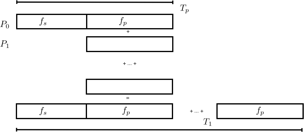
FIGURE 2.5: Sequential and parallel time in Gustafson's analysis.

(See figure  2.5  .) This is: \begin{equation} T_1=F_sT+p\cdot F_pT. \end{equation} This gives us a speedup of \begin{equation} S_p=\frac{T_1}{T_p}=\frac{F_s+p\cdot F_p}{F_s+F_p} = F_s+p\cdot F_p = p-(p-1)\cdot F_s. \label{eq:gustaf-s} \end{equation}

From this formula we see that:

• Speedup is still bounded by $p$;
• \ldots but it's a positive number;
• for a given $p$ it's again a decreasing function of the sequential fraction.

Exercise 2.5 and $F_p$. What is the asymptotic behavior of the efficiency $E_p$?
End of exercise

As with Amdahl's law, we can investigate the behavior of Gustafson's law if we include communication overhead. Let's go back to 2.2.3.1 problem, and approximate it as \begin{equation} S_p = p(1-\frac{T_c}{T_1}p). \end{equation} Now, under the assumption of a problem that is gradually being scaled up, $T_c$ and $T_1$ become functions of $p$. We see that, if $T_1(p)\sim pT_c(p)$, we get linear speedup that is a constant fraction away from $1$. As a general discussion we can not take this analysis further; in section  6.2.3 you'll see a detailed analysis of an example.

2.2.3.3 Amdahl's law and hybrid programming

crumb trail: > parallel > Theoretical concepts > Amdahl's law > Amdahl's law and hybrid programming

Above, you learned about hybrid programming, a mix between distributed and shared memory programming. This leads to a new form of Amdahl's law.

Suppose we have $p$ nodes with $c$ cores each, and $F_p$ describes the fraction of the code that uses $c$-way thread parallelism. We assume that the whole code is fully parallel over the $p$ nodes. The ideal speed up would be $p c$, and the ideal parallel running time $T_1/(pc)$, but the actual running time is \begin{equation} T_{p,c} = T_1 \left(\frac {F_s}{p} + \frac{F_p}{p c}\right) = \frac{T_1}{pc}\left( F_sc+F_p\right) = \frac{T_1}{pc}\left( 1+ F_s(c-1)\right). \end{equation}

Exercise Show that the speedup $T_1/T_{p,c}$ can be approximated by $p/F_s$.
End of exercise

In the original Amdahl's law, speedup was limited by the sequential portion to a fixed number $1/F_s$, in hybrid programming it is limited by the task parallel portion to $p/F_s$.

2.2.4 Critical path and Brent's theorem

crumb trail: > parallel > Theoretical concepts > Critical path and Brent's theorem

The above definitions of speedup and efficiency, and the discussion of Amdahl's law and Gustafson's law, made an implicit assumption that parallel work can be arbitrarily subdivided. As you saw in the summing example in section  2.1  , this may not always be the case: there can be dependencies between operations, meaning that one operation depends on an earlier in the sense of needing its result as input. Dependent operations can not be executed simultaneously, so they limit the amount of parallelism that can be employed.

We define the critical path as a (possibly non-unique) chain of dependencies of maximum length. (This length is sometimes known as  span  .) Since the tasks on a critical path need to be executed one after another, the length of the critical path is a lower bound on parallel execution time.

To make these notions precise, we define the following concepts:

Definition \begin{equation} \begin{array}{l@{\colon}l} T_1&\hbox{the time the computation takes on a single processor}\\ T_p&\hbox{the time the computation takes with $p$ processors}\\ T_\infty&\hbox{the time the computation takes if unlimited processors are available}\\ P_\infty&\hbox{the value of $p$ for which $T_p=T_\infty$} \end{array} \end{equation}
End of definition

With these concepts, we can define the average parallelism of an algorithm as $T_1/T_\infty$, and the length of the critical path is $T_\infty$.

We will now give a few illustrations by showing a graph of tasks and their dependencies. We assume for simplicity that each node is a unit time task.

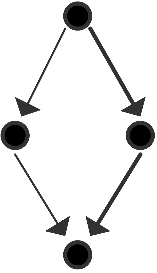
The maximum number of processors that can be used is 2 and the average parallelism is $4/3$: \begin{equation} \begin{array}{l} T_1=4,\quad T_\infty=3 \quad\Rightarrow T_1/T_\infty=4/3\\ T_2=3,\quad S_2=4/3,\quad E_2=2/3\\ P_\infty=2 \end{array} \end{equation}

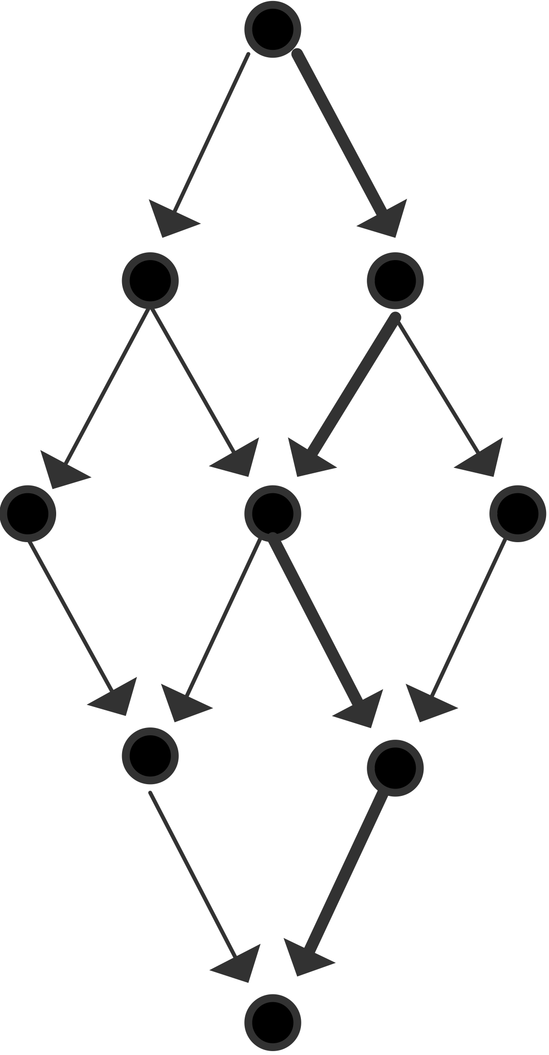
The maximum number of processors that can be used is 3 and the average parallelism is $9/5$; efficiency is maximal for $p=2$: \begin{equation} \begin{array}{l} T_1=9,\quad T_\infty=5 \quad\Rightarrow T_1/T_\infty=9/5\\ T_2=6,\quad S_2=3/2,\quad E_2=3/4\\ T_3=5,\quad S_3=9/5,\quad E_3=3/5\\ P_\infty=3 \end{array} \end{equation}

The maximum number of processors that can be used is 4 and that is also the average parallelism; the figure illustrates a parallelization with $P=3$ that has efficiency $\equiv1$: \begin{equation} \begin{array}{l} T_1=12,\quad T_\infty=4 \quad\Rightarrow T_1/T_\infty=3\\ T_2=6,\quad S_2=2,\quad E_2=1\\ T_3=4,\quad S_3=3,\quad E_3=1\\ T_4=3,\quad S_4=4,\quad E_4=1\\ P_\infty=4 \end{array} \end{equation}

Based on these examples, you probably see that there are two extreme cases:

• If every task depends on precisely on other, you get a chain of dependencies, and $T_p=T_1$ for any $p$.
• On the other hand, if all tasks are independent (and $p$ divides their number) you get $T_p=T_1/p$ for any $p$.
• In a slightly less trivial scenario than the previous, consider the case where the critical path is of length $m$, and in each of these $m$ steps there are $p-1$ independent tasks, or at least: dependent only on tasks in the previous step. There will then be perfect parallelism in each of the $m$ steps, and we can express $T_p = T_1/p$ or $T_p= m+ (T_1-m)/p$.

That last statement actually holds in general. This is known as Brent's theorem :

Theorem Let $m$ be the total number of tasks, $p$ the number of processors, and $t$ the length of a critical path  . Then the computation can be done in \begin{equation} T_p \leq t +\frac{m-t}{p}. \end{equation}
End of theorem

Proof Divide the computation in steps, such that tasks in step $i+1$ are independent of each other, and only dependent on step $i$. Let $s_i$ be the number of tasks in step $i$, then the time for that step is $\lceil \frac{s_i}{p} \rceil$. Summing over $i$ gives \begin{equation} T_p = \sum_i^t \lceil \frac{s_i}{p} \rceil \leq \sum_i^t \frac{s_i+p-1}{p} = t + \sum_i^t \frac{s_i-1}{p} = t+\frac{m-t}{p}. \end{equation}
End of proof

Exercise Consider a tree of depth $d$, that is, with $2^d-1$ nodes, and a search \begin{equation} \max_{n\in\mathrm{nodes}} f(n). \end{equation} Assume that all nodes need to be visited: we have no knowledge or any ordering on their values.

Analyze the parallel running time on $p$ processors, where you may assume that $p=2^q$, with $q
End of exercise

Exercise Apply Brent's theorem to Gaussian elimination, assuming that add/multiply/division all take one unit time.

Describe the critical path and give the length. What is the resulting upper bound on the parallel runtime?

How many processors could you theoretically use? What speedup and efficiency does that give?
End of exercise

2.2.5 Scalability

crumb trail: > parallel > Theoretical concepts > Scalability

Above, we remarked that splitting a given problem over more and more processors does not make sense: at a certain point there is just not enough work for each processor to operate efficiently. Instead, in practice users of a parallel code will either choose the number of processors to match the problem size, or they will solve a series of increasingly larger problems on correspondingly growing numbers of processors. In both cases it is hard to talk about speedup. Instead, the concept of scalability is used.

We distinguish two types of scalability. So-called strong scalability is in effect the same as speedup as discussed above. We say that a problem shows strong scalability if, partitioned over more and more processors, it shows perfect or near perfect speedup, that is, the execution time goes down linearly with the number of processors. In terms of efficiency we can describe this as: \begin{equation} \left. \begin{array}{l} N\equiv\mathrm{constant}\\ P\rightarrow\infty \end{array} \right\} \Rightarrow E_P\approx\mathrm{constant} \end{equation} Typically, one encounters statements like `this problem scales up to 500 processors', meaning that up to 500 processors the speedup will not noticeably decrease from optimal. It is not necessary for this problem to fit on a single processor: often a smaller number such as 64 processors is used as the baseline from which scalability is judged.

Exercise We can formulate strong scaling as a runtime that is inversely proportional to the number of processors: \begin{equation} t=c/p. \end{equation} Show that on a log-log plot, that is, you plot the logarithm of the runtime against the logarithm of the number of processors, you will get a straight line with slope $-1$.

Can you suggest a way of dealing with a non-parallelizable section, that is, with a runtime $t=c_1+c_2/p$?
End of exercise

More interestingly, weak scalability describes the behavior of execution as problem size and number of processors both grow, but in such a way that the amount of work per processor stays constant. The term `work' here is ambiguous: sometimes weak scaling is interpreted as keeping the amount of data constant, in other cases it's the number of operations that stays constant.

Measures such as speedup are somewhat hard to report, since the relation between the number of operations and the amount of data can be complicated. If this relation is linear, one could state that the amount of data per processor is kept constant, and report that parallel execution time is constant as the number of processors grows. (Can you think of applications where the relation between work and data is linear? Where it is not?)

In terms of efficiency: \begin{equation} \left. \begin{array}{l} N\rightarrow\infty\\ P\rightarrow\infty\\ M=N/P\equiv\mathrm{constant} \end{array} \right\} \Rightarrow E_P\approx\mathrm{constant} \end{equation}

Exercise Suppose you are investigating the weak scalability of a code. After running it for a couple of sizes and corresponding numbers of processes, you find that in each case the flop rate is roughly the same. Argue that the code is indeed weakly scalable.
End of exercise

Exercise In the above discussion we always implicitly compared a sequential algorithm and the parallel form of that same algorithm. However, in section  2.2.1 we noted that sometimes speedup is defined as a comparison of a parallel algorithm with the \textbf{best} sequential algorithm for the same problem. With that in mind, compare a parallel sorting algorithm with runtime $(\log n)^2$ (for instance, bitonic sort ; section  8.6  ) to the best serial algorithm, which has a running time of $n\log n$.

Show that in the weak scaling case of $n=p$ speedup is $p/\log p$. Show that in the strong scaling case speedup is a descending function of $n$.
End of exercise

Remark A historical anecdote.

Message:  1023110, 88 lines Posted:  5:34pm EST, Mon Nov
25/85, imported:  ....  Subject:  Challenge from Alan Karp
To:  Numerical-Analysis, ...  From GOLUB@SU-SCORE.ARPA

I have just returned from the Second SIAM Conference on
Parallel Processing for Scientific Computing in Norfolk,
Virginia.  There I heard about 1,000 processor systems,
4,000 processor systems, and even a proposed 1,000,000
processor system.  Since I wonder if such systems are the
best way to do general purpose, scientific computing, I am
making the following offer.

I will pay $100 to the first person to demonstrate a speedup
of at least 200 on a general purpose, MIMD computer used for
scientific computing.  This offer will be withdrawn at 11:59
PM on 31 December 1995.

This was satisfied by scaling up the problem.
End of remark

2.2.5.1 Iso-efficiency

crumb trail: > parallel > Theoretical concepts > Scalability > Iso-efficiency

In the definition of weak scalability above, we stated that, under some relation between problem size $N$ and number of processors $P$, efficiency will stay constant. We can make this precise and define the iso-efficiency curve as the relation between $N,P$ that gives constant efficiency  [Grama:1993:isoefficiency]  .

2.2.5.2 Precisely what do you mean by scalable?

crumb trail: > parallel > Theoretical concepts > Scalability > Precisely what do you mean by scalable?

In scientific computing scalability is a property of an algorithm and the way it is parallelized on an architecture, in particular noting the way data is distributed.

In computer industry parlance the term `scalability' is sometimes applied to architectures or whole computer systems:

A scalable computer is a computer designed from a small number of basic components, without a single bottleneck component, so that the computer can be incrementally expanded over its designed scaling range, delivering linear incremental performance for a well-defined set of scalable applications. General-purpose scalable computers provide a wide range of processing, memory size, and I/O resources. Scalability is the degree to which performance increments of a scalable computer are linear''  [Bell:outlook]  .

In particular,

• horizontal scaling is adding more hardware components, such as adding nodes to a cluster;
• vertical scaling corresponds to using more powerful hardware, for instance by doing a hardware upgrade.

2.2.6 Simulation scaling

crumb trail: > parallel > Theoretical concepts > Simulation scaling

In most discussions of weak scaling we assume that the amount of work and the amount of storage are linearly related. This is not always the case; for instance the operation complexity of a matrix-matrix product is $N^3$ for $N^2$ data. If you linearly increase the number of processors, and keep the data per process constant, the work may go up with a higher power.

A similar effect comes into play if you simulate time-dependent PDEs  . (This uses concepts from chapter  Numerical treatment of differential equations  .) Here, the total work is a product of the work per time step and the number of time steps. These two numbers are related; in section  4.1.2 you will see that the time step has a certain minimum size as a function of the space discretization. Thus, the number of time steps will go up as the work per time step goes up.

Consider now applications such as weather prediction  , and say that currently you need 4 hours of compute time to predict the next 24 hours of weather. The question is now: if you are happy with these numbers, and you buy a bigger computer to get a more accurate prediction, what can you say about the new computer?

In other words, rather than investigating scalability from the point of the running of an algorithm, in this section we will look at the case where the simulated time $S$ and the running time $T$ are constant. Since the new computer is presumably faster, we can do more operations in the same amount of running time. However, it is not clear what will happen to the amount of data involved, and hence the memory required. To analyze this we have to use some knowledge of the math of the applications.

Let $m$ be the memory per processor, and $P$ the number of processors, giving: \begin{equation} M=Pm\qquad\hbox{total memory.} \end{equation} If $d$ is the number of space dimensions of the problem, typically 2 or 3, we get \begin{equation} \Delta x = 1/M^{1/d}\qquad\hbox{grid spacing.} \end{equation} For stability this limits the time step $\Delta t$ to \begin{equation} \Delta t= \begin{cases} \Delta x=1\bigm/M^{1/d}&\hbox{hyperbolic case}\\ \Delta x^2=1\bigm/M^{2/d}&\hbox{parabolic case} \end{cases} \end{equation} (noting that the hyperbolic case was not discussed in chapter  Numerical treatment of differential equations  .) With a simulated time $S$, we find \begin{equation} k=S/\Delta t\qquad \hbox{time steps.} \end{equation} If we assume that the individual time steps are perfectly parallelizable, that is, we use explicit methods, or implicit methods with optimal solvers, we find a running time \begin{equation} T=kM/P=\frac{S}{\Delta t}m. \end{equation} Setting $T/S=C$, we find \begin{equation} m=C\Delta t, \end{equation} that is, the amount of memory per processor goes down as we increase the processor count. (What is the missing step in that last sentence?)

Further analyzing this result, we find \begin{equation} m=C\Delta t = c \begin{cases} 1\bigm/M^{1/d}&\hbox{hyperbolic case}\\ 1\bigm/M^{2/d}&\hbox{parabolic case} \end{cases} \end{equation} Substituting $M=Pm$, we find ultimately \begin{equation} m = C \begin{cases} 1\bigm/P^{1/(d+1)}&\hbox{hyperbolic}\\ 1\bigm/P^{2/(d+2)}&\hbox{parabolic} \end{cases} \end{equation} that is, the memory per processor that we can use goes down as a higher power of the number of processors.

Exercise Explore simulation scaling in the context of the Linpack benchmark  , that is, Gaussian elimination. Ignore the system solving part and only consider the factorization part; assume that it can be perfectly parallelized.

1. Suppose you have a single core machine, and your benchmark run takes time $T$ with $M$ words of memory. Now you buy a processor twice as fast, and you want to do a benchmark run that again takes time $T$. How much memory do you need?
2. Now suppose you have a machine with $P$ processors, each with $M$ memory, and your benchmark run takes time $T$. You buy a machine with $2P$ processors, of the same clock speed and core count, and you want to do a benchmark run, again taking time $T$. How much memory does each node take?

End of exercise

2.2.7 Other scaling measures

crumb trail: > parallel > Theoretical concepts > Other scaling measures

Amdahl's law above was formulated in terms of the execution time on one processor. In many practical situations this is unrealistic, since the problems executed in parallel would be too large to fit on any single processor. Some formula manipulation gives us quantities that are to an extent equivalent, but that do not rely on this single-processor number  [Moreland:formalmetrics2015]  .

For starters, applying the definition $S_p(n) = \frac{ T_1(n) }{ T_p(n) }$ to strong scaling, we observe that $T_1(n)/n$ is the sequential time per operation, and its inverse $n/T_1(n)$ can be called the sequential computational rate  , denoted $R_1(n)$. Similarly defining a `parallel computational rate' \begin{equation} R_p(n) = n/T_p(n) \end{equation} we find that \begin{equation} S_p(n) = R_p(n)/R_1(n) \end{equation} In strong scaling $R_1(n)$ will be a constant, so we make a logarithmic plot of speedup, purely based on measuring $T_p(n)$.

2.2.8 Concurrency; asynchronous and distributed computing

crumb trail: > parallel > Theoretical concepts > Concurrency; asynchronous and distributed computing

Even on computers that are not parallel there is a question of the execution of multiple simultaneous processes. Operating systems typically have a concept of time slicing  , where all active process are given command of the CPU for a small slice of time in rotation. In this way, a sequential can emulate a parallel machine; of course, without the efficiency.

However, time slicing is useful even when not running a parallel application: OSs will have independent processes (your editor, something monitoring your incoming mail, et cetera) that all need to stay active and run more or less often. The difficulty with such independent processes arises from the fact that they sometimes need access to the same resources. The situation where two processes both need the same two resources, each getting hold of one, is called deadlock  . A famous formalization of resource contention is known as the dining philosophers problem.

The field that studies such as independent processes is variously known as concurrency  , asynchronous computing  , or distributed computing  . The term concurrency describes that we are dealing with tasks that are simultaneously active, with no temporal ordering between their actions. The term distributed computing derives from such applications as database systems, where multiple independent clients need to access a shared database.

We will not discuss this topic much in this book. Section  2.6.1 discusses the thread mechanism that supports time slicing; on modern multicore processors threads can be used to implement shared memory parallel computing.

The book `Communicating Sequential Processes' offers an analysis of the interaction between concurrent processes  [Hoare:CSP]  . Other authors use topology to analyze asynchronous computing  [Herlihy:1999:topological]  .

2.3 Parallel Computers Architectures

crumb trail: > parallel > Parallel Computers Architectures

For quite a while now, the top computers have been some sort of parallel computer, that is, an architecture that allows the simultaneous execution of multiple instructions or instruction sequences. One way of characterizing the various forms this can take is due to Flynn  [flynn:taxonomy]  . Flynn's taxonomy characterizes architectures by whether the data flow and control flow are shared or independent. The following four types result (see also figure  2.6  ):

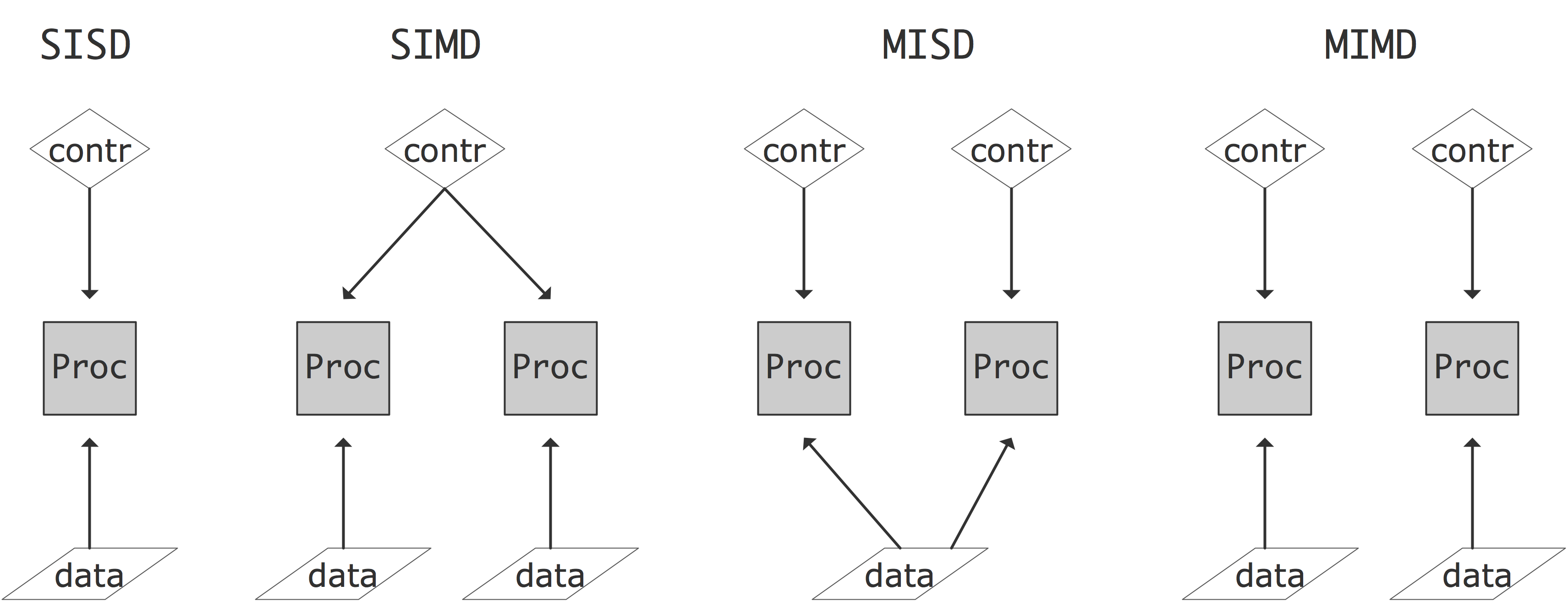
FIGURE 2.6: The four classes of the Flynn's taxonomy.

• [SISD] Single Instruction Single Data: this is the traditional CPU architecture: at any one time only a single instruction is executed, operating on a single data item.
• [SIMD] Single Instruction Multiple Data: in this computer type there can be multiple processors, each operating on its own data item, but they are all executing the same instruction on that data item. Vector computers (section  2.3.1.1  ) are typically also characterized as SIMD.
• [MISD] Multiple Instruction Single Data. No architectures answering to this description exist; one could argue that redundant computations for safety-critical applications are an example of MISD.
• [MIMD] Multiple Instruction Multiple Data: here multiple CPUs operate on multiple data items, each executing independent instructions. Most current parallel computers are of this type.

We will now discuss SIMD and MIMD architectures in more detail.

\newpage

2.3.1 SIMD

crumb trail: > parallel > Parallel Computers Architectures > SIMD

WRAPFIGURE 2.7: Architecture of the MasPar 2 array processor.

Parallel computers of the SIMD type apply the same operation simultaneously to a number of data items. The design of the CPUs of such a computer can be quite simple, since the arithmetic unit does not need separate logic and instruction decoding units: all CPUs execute the same operation in lock step. This makes SIMD computers excel at operations on arrays, such as

for (i=0; i<N; i++) a[i] = b[i]+c[i];

and, for this reason, they are also often called \indexterm{array processors}. Scientific codes can often be written so that a large fraction of the time is spent in array operations.

On the other hand, there are operations that can not can be executed efficiently on an array processor. For instance, evaluating a number of terms of a recurrence $x_{i+1}=ax_i+b_i$ involves that many additions and multiplications, but they alternate, so only one operation of each type can be processed at any one time. There are no arrays of numbers here that are simultaneously the input of an addition or multiplication.

In order to allow for different instruction streams on different parts of the data, the processor would have a `mask bit' that could be set to prevent execution of instructions. In code, this typically looks like

where (x>0) {
  x[i] = sqrt(x[i])

The programming model where identical operations are applied to a number of data items simultaneously, is known as data parallelism  .

Such array operations can occur in the context of physics simulations, but another important source is graphics applications. For this application, the processors in an array processor can be much weaker than the processor in a PC: often they are in fact bit processors, capable of operating on only a single bit at a time. Along these lines, ICL had the 4096 processor DAP  [DAP:79a] in the 1980s, and Goodyear MPP  [Batcher:85a] in the 1970s.

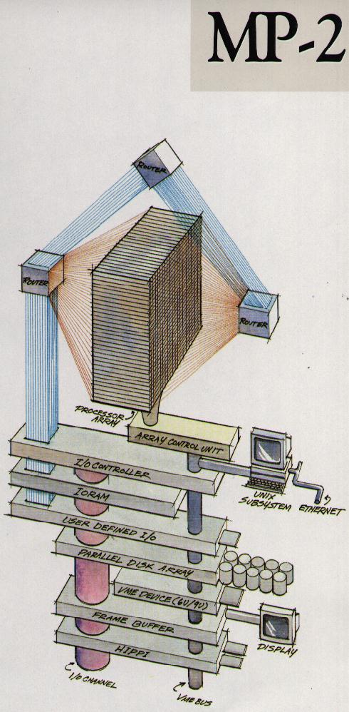
Later, the Connection Machine (CM-1, CM-2, CM-5) were quite popular. While the first Connection Machine had bit processors (16 to a chip), the later models had traditional processors capable of floating point arithmetic, and were not true SIMD architectures. All were based on a hyper-cube interconnection network; see section  2.7.5  . Another manufacturer that had a commercially successful array processor was MasPar ; figure  2.7 illustrates the architecture. You clearly see the single control unit for a square array of processors, plus a network for doing global operations.

Supercomputers based on array processing do not exist anymore, but the notion of SIMD lives on in various guises. For instance, GPUs are SIMD-based, enforced through their CUDA programming language. Also, the Intel Xeon Phi has a strong SIMD component. While early SIMD architectures were motivated by minimizing the number of transistors necessary, these modern co-processors are motivated by power efficiency considerations. Processing instructions (known as instruction issue  ) is actually expensive compared to a floating point operation, in time, energy, and chip real estate needed. Using SIMD is then a way to economize on the last two measures.

2.3.1.1 Pipelining and pipeline processors

crumb trail: > parallel > Parallel Computers Architectures > SIMD > Pipelining and pipeline processors

A number of computers have been based on a \indexterm{vector processor} or pipeline processor design. The first commercially successful supercomputers, the Cray-1 and the Cyber-205 were of this type. In recent times, the Cray-X1 and the NEC SX series have featured vector pipes. The `Earth Simulator' computer  [Sato2004]  , which led the TOP500 (section  2.11.6  ) for 3 years, was based on NEC SX processors. The general idea behind pipelining was described in section  1.2.1.3  .

While supercomputers based on pipeline processors are in a distinct minority, pipelining is now mainstream in the superscalar CPUs that are the basis for clusters  . A typical CPU has pipelined floating point units, often with separate units for addition and multiplication; see section  1.2.1.3  .

However, there are some important differences between pipelining in a modern superscalar CPU and in, more old-fashioned, vector units. The pipeline units in these vector computers are not integrated floating point units in the CPU, but can better be considered as attached vector units to a CPU that itself has a floating point unit. The vector unit has vector registers

(Note: {The Cyber205 was an exception, with direct-to-memory architecture.}  )

with a typical length of 64 floating point numbers; there is typically no `vector cache'. The logic in vector units is also simpler, often addressable by explicit vector instructions. Superscalar CPUs, on the other hand, are fully integrated in the CPU and geared towards exploiting data streams in unstructured code.

2.3.1.2 True SIMD in CPUs and GPUs

crumb trail: > parallel > Parallel Computers Architectures > SIMD > True SIMD in CPUs and GPUs

True SIMD array processing can be found in modern CPUs and GPUs, in both cases inspired by the parallelism that is needed in graphics applications.

Modern CPUs from Intel and AMD, as well as PowerPC chips, have \indextermbusdef{vector}{instructions} that can perform multiple instances of an operation simultaneously. On Intel processors this is known as SSE or AVX  . These extensions were originally intended for graphics processing, where often the same operation needs to be performed on a large number of pixels. Often, the data has to be a total of, say, 128 bits, and this can be divided into two 64-bit reals, four 32-bit reals, or a larger number of even smaller chunks such as 4 bits.

The AVX instructions are based on up to 512-bit wide SIMD, that is, eight double precision floating point numbers can be processed simultaneously. Just as single floating point operations operate on data in registers (section  1.3.3  ), vector operations use vector registers  . The locations in a vector register are sometimes referred to as \indextermbusdef{SIMD}{lanes}.

The use of SIMD is mostly motivated by power considerations. Decoding instructions can be more power consuming than executing them, so SIMD parallelism is a way to save power.

Current compilers can generate SSE or AVX instructions automatically; sometimes it is also possible for the user to insert pragmas, for instance with the Intel compiler:

void func(float *restrict c, float *restrict a,
          float *restrict b, int n)
{
#pragma vector always
  for (int i=0; i<n; i++)
    c[i] = a[i] * b[i];
}

Use of these extensions often requires data to be aligned with cache line boundaries (section  1.3.4.7  ), so there are special allocate and free calls that return aligned memory.

Version 4 of OpenMP also has directives for indicating SIMD parallelism.

Array processing on a larger scale can be found in GPU s. A  GPU contains a large number of simple processors, ordered in groups of 32, typically. Each processor group is limited to executing the same instruction. Thus, this is true example of  SIMD processing. For further discussion, see section  2.9.3  .

2.3.2 MIMD / SPMD computers

crumb trail: > parallel > Parallel Computers Architectures > MIMD / SPMD computers

By far the most common parallel computer architecture these days is called MIMD : the processors execute multiple, possibly differing instructions, each on their own data. Saying that the instructions differ does not mean that the processors actually run different programs: most of these machines operate in SPMD mode, where the programmer starts up the same executable on the parallel processors. Since the different instances of the executable can take differing paths through conditional statements, or execute differing numbers of iterations of loops, they will in general not be completely in sync as they were on SIMD machines. If this lack of synchronization is due to processors working on different amounts of data, it is called load unbalance  , and it is a major source of less than perfect speedup ; see section  2.10  .

There is a great variety in MIMD computers. Some of the aspects concern the way memory is organized, and the network that connects the processors. Apart from these hardware aspects, there are also differing ways of programming these machines. We will see all these aspects below. Many machines these days are called clusters  . They can be built out of custom or commodity processors (if they consist of PCs, running Linux, and connected with Ethernet  , they are referred to as \indextermsub{Beowulf} {clusters}  [Gropp:BeowulfBook]  ); since the processors are independent they are examples of the MIMD or SPMD model.

2.3.3 The commoditization of supercomputers

crumb trail: > parallel > Parallel Computers Architectures > The commoditization of supercomputers

In the 1980s and 1990s supercomputers were radically different from personal computer and mini or super-mini computers such as the DEC PDP and VAX series. The SIMD vector computers had one ( CDC Cyber205 or Cray-1  ), or at most a few ( ETA-10  , Cray-2  , Cray X/MP  , Cray Y/MP  ), extremely powerful processors, often a vector processor. Around the mid-1990s clusters with thousands of simpler (micro) processors started taking over from the machines with relative small numbers of vector pipes (see http://www.top500.org/lists/1994/11  ). At first these microprocessors ( IBM Power series  , Intel i860  , MIPS  , DEC Alpha  ) were still much more powerful than `home computer' processors, but later this distinction also faded to an extent. Currently, many of the most powerful clusters are powered by essentially the same Intel Xeon and AMD Opteron chips that are available on the consumer market. Others use IBM Power Series or other `server' chips. See section  2.11.6 for illustrations of this history since 1993.

2.4 Different types of memory access

crumb trail: > parallel > Different types of memory access

In the introduction we defined a parallel computer as a setup where multiple processors work together on the same problem. In all but the simplest cases this means that these processors need access to a joint pool of data. In the previous chapter you saw how, even on a single processor, memory can have a hard time keeping up with processor demands. For parallel machines, where potentially several processors want to access the same memory location, this problem becomes even worse. We can characterize parallel machines by the approach they take to the problem of reconciling multiple accesses, by multiple processes, to a joint pool of data.

The main distinction here is between distributed memory and shared memory  . With distributed memory, each processor has its own physical memory, and more importantly its own address space  .

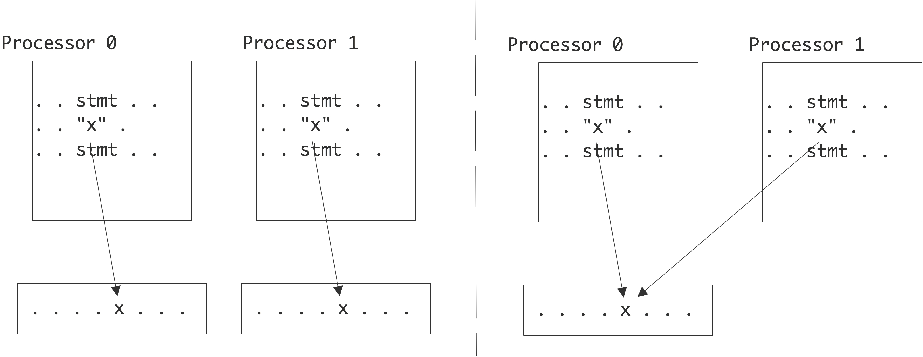\caption{References to identically named variables in the distributed and shared memory case.}

Thus, if two processors refer to a variable  x  , they access a variable in their own local memory. This is an instance of the SPMD model.

On the other hand, with shared memory, all processors access the same memory; we also say that they have a shared address space  . See figure  2.4  .

2.4.1 Symmetric Multi-Processors: Uniform Memory Access

crumb trail: > parallel > Different types of memory access > Symmetric Multi-Processors: Uniform Memory Access

Parallel programming is fairly simple if any processor can access any memory location. For this reason, there is a strong incentive for manufacturers to make architectures where processors see no difference between one memory location and another: any memory location is accessible to every processor, and the access times do not differ. This is called UMA  , and the programming model for architectures on this principle is often called SMP  .

There are a few ways to realize an SMP architecture. Current desktop computers can have a few processors accessing a shared memory through a single memory bus; for instance Apple markets a model with 2 six-core processors. Having a memory bus that is shared between processors works only for small numbers of processors; for larger numbers one can use a crossbar that connects multiple processors to multiple memory banks; see section  2.7.6  . 2.21 shows 2.7.6.2 show butterfly exchange  , which is built up out of simple

On multicore processors there is uniform memory access of a different type: the cores typically have a shared cache  , typically the L3 or L2 cache.

2.4.2 Non-Uniform Memory Access

crumb trail: > parallel > Different types of memory access > Non-Uniform Memory Access

The UMA approach based on shared memory is obviously limited to a small number of processors. The crossbar networks are expandable, so they would seem the best choice. However, in practice one puts processors with a local memory in a configuration with an exchange network. This leads to a situation where a processor can access its own memory fast, and other processors' memory slower. This is one case of so-called NUMA : a strategy that uses physically distributed memory, abandoning the uniform access time, but maintaining the logically shared address space: each processor can still access any memory location.

2.4.2.1 Affinity

crumb trail: > parallel > Different types of memory access > Non-Uniform Memory Access > Affinity

When we have NUMA  , the question of where to place data, in relation to the process or thread that will access it, becomes important. This is known as affinity ; if we look at it from the point of view of placing the processes or threads, it is called process affinity  .

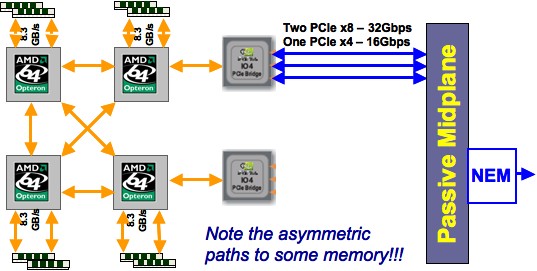
QUOTE 2.8: Non-uniform memory access in a four-socket motherboard.

Figure  2.8 illustrates NUMA in the case of the four-socket motherboard of the TACC Ranger cluster  . Each chip has its own memory (8Gb) but the motherboard acts as if the processors have access to a shared pool of 32Gb. Obviously, accessing the memory of another processor is slower than accessing local memory. In addition, note that each processor has three connections that could be used to access other memory, but the rightmost two chips use one connection to connect to the network. This means that accessing each other's memory can only happen through an intermediate processor, slowing down the transfer, and tying up that processor's connections.

2.4.2.2 Coherence

crumb trail: > parallel > Different types of memory access > Non-Uniform Memory Access > Coherence

While the NUMA approach is convenient for the programmer, it offers some challenges for the system. Imagine that two different processors each have a copy of a memory location in their local (cache) memory. If one processor alters the content of this location, this change has to be propagated to the other processors. If both processors try to alter the content of the one memory location, the behavior of the program can become undetermined.

Keeping copies of a memory location synchronized is known as cache coherence (see section  1.4.1 for further details); a multi-processor system using it is sometimes called a `cache-coherent NUMA' or ccNUMA architecture.

Taking NUMA to its extreme, it is possible to have a software layer that makes network-connected processors appear to operate on shared memory. This is known as distributed shared memory or virtual shared memory  . In this approach a hypervisor offers a shared memory API, by translating system calls to distributed memory management. This shared memory API can be utilized by the Linux kernel  , which can support 4096 threads.

Among current vendors only SGI (the UV line) and Cray (the XE6  ) market products with large scale NUMA. Both offer strong support for PGAS languages; see section  2.6.5  . There are vendors, such as ScaleMP  , that offer a software solution to distributed shared memory on regular clusters.

2.4.3 Logically and physically distributed memory

crumb trail: > parallel > Different types of memory access > Logically and physically distributed memory

The most extreme solution to the memory access problem is to offer memory that is not just physically, but that is also logically distributed: the processors have their own address space, and can not directly see another processor's memory. This approach is often called `distributed memory', but this term is unfortunate, since we really have to consider the questions separately whether memory is distributed and whether is appears distributed. Note that NUMA also has physically distributed memory; the distributed nature of it is just not apparent to the programmer.

With logically and physically distributed memory, the only way one processor can exchange information with another is through passing information explicitly through the network. You will see more about this in section  2.6.3.3  .

This type of architecture has the significant advantage that it can scale up to large numbers of processors: the IBM BlueGene has been built with over 200,000 processors. On the other hand, this is also the hardest kind of parallel system to program.

Various kinds of hybrids between the above types exist. In fact, most modern clusters will have NUMA nodes, but a distributed memory network between nodes.

2.5 Granularity of parallelism

crumb trail: > parallel > Granularity of parallelism

In this section we look at parallelism from a point of how far to subdivide the work over processing elements. The concept we explore here is that of granularity : the balance between the amount of independent work per processing element, and how often processing elements need to synchronize. We talk of `large grain parallelism' if there is a lot of work in between synchronization points, and `small grain parallelism' if that amount of work is small. Obviously, in order for small grain parallelism to be profitable, the synchronization needs to be fast; with large grain parallelism we can tolerate most costly synchronization.

The discussion in this section will be mostly on a conceptual level; in section  2.6 we will go into some detail on actual parallel programming.

2.5.1 Data parallelism

crumb trail: > parallel > Granularity of parallelism > Data parallelism

It is fairly common for a program to have loops with a simple body that gets executed for all elements in a large data set:

for (i=0; i<1000000; i++)
  a[i] = 2*b[i];

Such code is considered an instance of data parallelism or fine-grained parallelism  . If you had as many processors as array elements, this code would look very simple: each processor would execute the statement

a = 2*b

on its local data.

If your code consists predominantly of such loops over arrays, it can be executed efficiently with all processors in lockstep. Architectures based on this idea, where the processors can in fact only work in lockstep, have existed, see section  2.3.1  . Such fully parallel operations on arrays appear in computer graphics, where every pixel of an image is processed independently. For this reason, GPUs (section  2.9.3  ) are strongly based on data parallelism.

The CUDA language, invented by NVidia  , allows for elegant expression of data parallelism. Later developed languages, such as Sycl  , or libraries such as Kokkos  , aim at similar expression, but are more geared towards heterogeneous parallelism.

Continuing the above example for a little bit, consider the operation

\begin{displayalgorithm} \For{$0\leq i<\mathrm{max}$}{ $i_{
mathrm{left}}=
mod(i-1,
mathrm{max})$

$i_{
mathrm{right}}=
mod(i+1,
mathrm{max})$

$a_i = (b_{i_{\mathrm{left}}}+b_{i_{\mathrm{right}}})/2$} \end{displayalgorithm}

On a data parallel machine, that could be implemented as

\begin{displayalgorithm} \SetKw{shiftleft}{shiftleft} \SetKw{shiftright}{shiftright} $ bleft \leftarrow \shiftright( b  )$

$ bright \leftarrow \shiftleft( b  )$

$ a \leftarrow ( bleft + bright  )/2$ \end{displayalgorithm}

where the shiftleft/right instructions cause a data item to be sent to the processor with a number lower or higher by 1. For this second example to be efficient, it is necessary that each processor can communicate quickly with its immediate neighbors, and the first and last processor with each other.

In various contexts such a `blur' operations in graphics, it makes sense to have operations on 2D data:

\begin{displayalgorithm} \For{$0

and consequently processors have be able to move data to neighbors in a 2D grid.

2.5.2 Instruction-level parallelism

crumb trail: > parallel > Granularity of parallelism > Instruction-level parallelism

In ILP  , the parallelism is still on the level of individual instructions, but these need not be similar. For instance, in

\begin{displayalgorithm} $a
leftarrow b+c$

$d
leftarrow e*f$ \end{displayalgorithm}

the two assignments are independent, and can therefore be executed simultaneously. This kind of parallelism is too cumbersome for humans to identify, but compilers are very good at this. In fact, identifying ILP is crucial for getting good performance out of modern superscalar CPUs.

2.5.3 Task-level parallelism

crumb trail: > parallel > Granularity of parallelism > Task-level parallelism

At the other extreme from data and instruction-level parallelism, task parallelism that can be executed in parallel. As an example, a search in a tree data structure could be implemented as follows:

{SearchInTree}{root} \SetKw{optimal}{optimal}\SetKw{exit}{exit}\SetKw{search}{SearchInTree}\SetKw{parl}{parallel} \eIf{\optimal(root)}{\exit} {\parl: \search(leftchild),\search(rightchild)}

The search tasks in this example are not synchronized, and the number of tasks is not fixed: it can grow arbitrarily. In practice, having too many tasks is not a good idea, since processors are most efficient if they work on just a single task. Tasks can then be scheduled as follows:

\begin{displayalgorithm} \While{there are tasks left}{ wait until a processor becomes inactive;

spawn a new task on it} \end{displayalgorithm}

(There is a subtle distinction between the two previous pseudo-codes. In the first, tasks were self-scheduling: each task spawned off two new ones. The second code is an example of the manager-worker paradigm : there is one central task which lives for the duration of the code, and which spawns and assigns the worker tasks.)

Unlike in the data parallel example above, the assignment of data to processor is not determined in advance in such a scheme. Therefore, this mode of parallelism is most suited for thread-programming, for instance through the OpenMP library; section  2.6.2  .

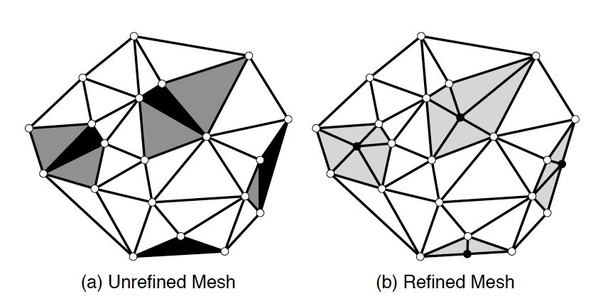
Let us consider a more serious example of task-level parallelism.

A finite element mesh is, in the simplest case, a collection of triangles that covers a 2D object. Since angles that are too acute should be avoided, the Delauney mesh refinement process can take certain triangles, and replace them by better shaped ones. This is illustrated in figure  2.9 : the black triangles violate some angle condition, so either they themselves get subdivided, or they are joined with some neighboring ones (rendered in grey) and then jointly redivided.

FIGURE 2.9: A mesh before and after refinement.

In pseudo-code, this can be implemented as in figure  2.10  .

\begin{displayalgorithm} Mesh m = /* read in initial mesh */

WorkList wl;

wl.add(mesh.badTriangles());

\While { (wl.size() != 0) } { Element e = wl.get(); //get bad triangle

if (e no longer in mesh) continue;

Cavity c = new Cavity(e);

c.expand();

c.retriangulate();

mesh.update(c);

wl.add(c.badTriangles());

} \end{displayalgorithm}

FIGURE 2.10: Task queue implementation of Delauney refinement.

(This figure and code are to be found in  [Kulkami:howmuch]  , which also contains a more detailed discussion.)

It is clear that this algorithm is driven by a worklist (or task queue  ) data structure that has to be shared between all processes. Together with the dynamic assignment of data to processes, this implies that this type of irregular parallelism is suited to shared memory programming, and is much harder to do with distributed memory.

2.5.4 Conveniently parallel computing

crumb trail: > parallel > Granularity of parallelism > Conveniently parallel computing

In certain contexts, a simple, often single processor, calculation needs to be performed on many different inputs. Since the computations have no data dependencies and need not be done in any particular sequence, this is often called embarrassingly parallel or \indexterm{conveniently parallel} computing. This sort of parallelism can happen at several levels. In examples such as calculation of the Mandelbrot set or evaluating moves in a chess game, a subroutine-level computation is invoked for many parameter values. On a coarser level it can be the case that a simple program needs to be run for many inputs. In this case, the overall calculation is referred to as a parameter sweep  .

2.5.5 Medium-grain data parallelism

crumb trail: > parallel > Granularity of parallelism > Medium-grain data parallelism

The above strict realization of data parallelism assumes that there are as many processors as data elements. In practice, processors will have much more memory than that, and the number of data elements is likely to be far larger than the processor count of even the largest computers. Therefore, arrays are grouped onto processors in subarrays. The code then looks like this:

my_lower_bound = // some processor-dependent number
my_upper_bound = // some processor-dependent number
for (i=my_lower_bound; i<my_upper_bound; i++)
  // the loop body goes here

This model has some characteristics of data parallelism, since the operation performed is identical on a large number of data items. It can also be viewed as task parallelism, since each processor executes a larger section of code, and does not necessarily operate on equal sized chunks of data.

2.5.6 Task granularity

crumb trail: > parallel > Granularity of parallelism > Task granularity

In the previous subsections we considered different level of finding parallel work, or different ways of dividing up work so as to find parallelism. There is another way of looking at this: we define the granularity of a parallel scheme as the amount of work (or the task size) that a processing element can perform before having to communicate or synchronize with other processing elements.

In ILP we are dealing with very fine-grained parallelism, on the order of a single instruction or just a few instructions. In true task parallelism the granularity is much coarser.

The interesting case here is data parallelism, where we have the freedom to choose the task sizes. On SIMD machines we can choose a granularity of a single instruction, but, as you saw in section  2.5.5  , operations can be grouped into medium-sized tasks. Thus, operations that are data parallel can be executed on distributed memory clusters, given the right balance between the number of processors and total problem size.

Exercise Discuss choosing the right granularity for a data parallel operation such as averaging on a two-dimensional grid. Show that there is a surface-to-volume effect: the amount of communication is of a lower order than the computation. This means that, even if communication is much slower than computation, increasing the task size will still give a balanced execution.
End of exercise

Unfortunately, choosing a large task size to overcome slow communication may aggravate another problem: aggregating these operations may give tasks with varying running time, causing load imbalance  . One solution here is to use an overdecomposition of the problem: create more tasks then there are processing elements, and assign multiple tasks to a processor (or assign tasks dynamically) to even out irregular running times. This is known as dynamic scheduling  , and the examples in section  2.5.3 illustrate this; see also section  2.6.2.1  . An example of overdecomposition in linear algebra is discussed in section  6.3.2  .

2.6 Parallel programming

crumb trail: > parallel > Parallel programming

Parallel programming is more complicated than sequential programming. While for sequential programming most programming languages operate on similar principles (some exceptions such as functional or logic languages aside), there is a variety of ways of tackling parallelism. Let's explore some of the concepts and practical aspects.

There are various approaches to parallel programming. First of all, there does not seem to be any hope of a parallelizing compiler that can automagically transform a sequential program into a parallel one. Apart from the problem of figuring out which operations are independent, the main problem is that the problem of locating data in a parallel context is very hard. A compiler would need to consider the whole code, rather than a subroutine at a time. Even then, results have been disappointing.

More productive is the approach where the user writes mostly a sequential program, but gives some indications about what computations can be parallelized, and how data should be distributed. Indicating parallelism of operations explicitly is done in OpenMP (section  2.6.2  ); indicating the data distribution and leaving parallelism to the compiler and runtime is the basis for PGAS languages (section  2.6.5  ). Such approaches work best with shared memory.

By far the hardest way to program in parallel, but with the best results in practice, is to expose the parallelism to the programmer and let the programmer manage everything explicitly. This approach is necessary in the case of distributed memory programming. We will have a general discussion of distributed programming in section  2.6.3.1 ; section  2.6.3.3 will discuss the MPI library.

2.6.1 Thread parallelism

crumb trail: > parallel > Parallel programming > Thread parallelism

As a preliminary to OpenMP (section  2.6.2  ), we will briefly go into `threads'.

To explain what a thread is, we first need to get technical about what a process is. A unix process corresponds to the execution of a single program. Thus, it has in memory:

• The program code, in the form of machine language instructions;
• A heap  , containing for instance arrays that were created with malloc ;
• A stack with quick-changing information, such as the program counter that indicates what instruction is currently being executed, and data items with local scope, as well as intermediate results from computations.

This process can have multiple threads; these are similar in that they see the same program code and heap, but they have their own stack. Thus, a thread is an independent `strand' of execution through a process.

Processes can belong to different users, or be different programs that a single user is running concurrently, so they have their own data space. On the other hand, threads are part of one process and therefore share the process heap. Threads can have some private data, for instance by have their own data stack, but their main characteristic is that they can collaborate on the same data.

2.6.1.1 The fork-join mechanism

crumb trail: > parallel > Parallel programming > Thread parallelism > The fork-join mechanism

Threads are dynamic, in the sense that they can be created during program execution. (This is different from the MPI model, where every processor run one process, and they are all created and destroyed at the same time.) When a program starts, there is one thread active: the main thread  . Other threads are created by \indextermbusdef{thread}{spawning}, and the main thread can wait for their completion.

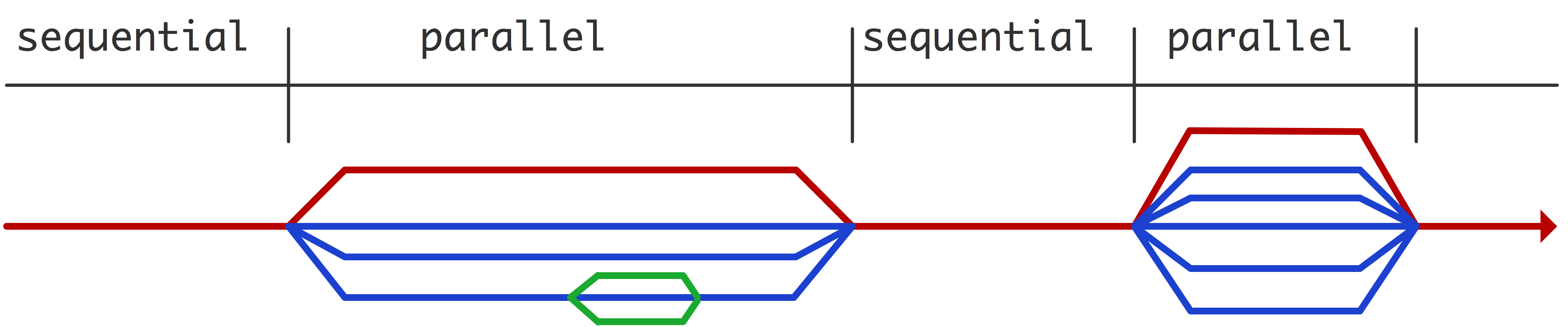
FIGURE 2.11: Thread creation and deletion during parallel execution.

This is known as the fork-join model; it is illustrated in figure  2.11  . A group of threads that is forked from the same thread and active simultaneously is known as a thread team  .

2.6.1.2 Hardware support for threads

crumb trail: > parallel > Parallel programming > Thread parallelism > Hardware support for threads

Threads as they were described above are a software construct. Threading was possible before parallel computers existed; they were for instance used to handle independent activities in an OS  . In the absence of parallel hardware, the OS would handle the threads through multitasking or \indextermdef{time slicing}: each thread would regularly get to use the CPU for a fraction of a second. (Technically, the Linux kernel treads processes and threads though the task concept; tasks are kept in a list, and are regularly activated or de-activated.)

This can lead to higher processor utilization, since the instructions of one thread can be processed while another thread is waiting for data. (On traditional CPUs, switching between threads is somewhat expensive (an exception is the hyperthreading mechanism) but on GPUs it is not, and in fact they need many threads to attain high performance.)

On modern multicore processors there is an obvious way of supporting threads: having one thread per core gives a parallel execution that uses your hardware efficiently. The shared memory allows the threads to all see the same data. This can also lead to problems; see section  2.6.1.5  .

2.6.1.3 Threads example

crumb trail: > parallel > Parallel programming > Thread parallelism > Threads example

The following example, which is strictly Unix-centric and will not work on Windows, is a clear illustration of the fork-join model. It uses the pthreads library to spawn a number of tasks that all update a global counter. Since threads share the same memory space, they indeed see and update the same memory location.

#include <stdlib.h>
#include <stdio.h>
#include "pthread.h"

int sum=0;

void adder() {
  sum = sum+1;
  return;
}

#define NTHREADS 50
int main() {
  int i;
  pthread_t threads[NTHREADS];
  printf("forking\n");
  for (i=0; i<NTHREADS; i++)
    if (pthread_create(threads+i,NULL,&adder,NULL)!=0) return i+1;
  printf("joining\n");
  for (i=0; i<NTHREADS; i++)
    if (pthread_join(threads[i],NULL)!=0) return NTHREADS+i+1;
  printf("Sum computed: %d\n",sum);

  return 0;
}

The fact that this code gives the right result is a coincidence: it only happens because updating the variable is so much quicker than creating the thread. (On a multicore processor the chance of errors will greatly increase.) If we artificially increase the time for the update, we will no longer get the right result:

void adder() {
  int t = sum; sleep(1); sum = t+1;
  return;
}

Now all threads read out the value of sum  , wait a while (presumably calculating something) and then update.

This can be fixed by having a lock on the code region that should be `mutually exclusive':

pthread_mutex_t lock;

void adder() {
  int t;
  pthread_mutex_lock(&lock);
  t = sum; sleep(1); sum = t+1; 
  pthread_mutex_unlock(&lock);
  return;
}

int main() {
  ....
  pthread_mutex_init(&lock,NULL);

The lock and unlock commands guarantee that no two threads can interfere with each other's update.

2.6.1.4 Contexts

crumb trail: > parallel > Parallel programming > Thread parallelism > Contexts

In the above example and its version with the sleep command we glanced over the fact that there were two types of data involved. First of all, the variable  s was created outside the thread spawning part. Thus, this variable was shared  .

On the other hand, the variable  t was created once in each spawned thread. We call this private data.

The totality of all data that a thread can access is called its context  . It contains private and shared data, as well as temporary results of computations that the thread is working on. (It also contains the program counter and stack pointer. If you don't know what those are, don't worry.)

It is quite possible to create more threads than a processor has cores, so a processor may need to switch between the execution of different threads. This is known as a \indextermbusdef{context}{switch}.

Context switches are not for free on regular CPUs, so they only pay off if the granularity of the threaded work is high enough. The exceptions to this story are:

• CPUs that have hardware support for multiple threads, for instance through hyperthreading (section  2.6.1.9  ), or as in the Intel Xeon Phi (section  2.9  );
• GPUs  , which in fact rely on fast context switching (section  2.9.3  );
• certain other `exotic' architectures such as the Cray XMT (section  2.8  ).

2.6.1.5 Race conditions, thread safety, and atomic operations

crumb trail: > parallel > Parallel programming > Thread parallelism > Race conditions, thread safety, and atomic operations

Shared memory makes life easy for the programmer, since every processor has access to all of the data: no explicit data traffic between the processor is needed. On the other hand, multiple processes/processors can also write to the same variable, which is a source of potential problems.

Suppose that two processes both try to increment an integer variable  I :

Init:
I=0

process 1:
I=I+2

process 2:
I=I+3

This is a legitimate activity if the variable is an accumulator for values computed by independent processes. The result of these two updates depends on the sequence in which the processors read and write the variable.

\toprule scenario 1.	scenario 1.	scenario 3.\ \midrule \multicolumn{6}{c}{$ I =0$}\ \midrule read $ I =0$	read $ I =0$	read $ I =0$	read $ I =0$	read $ I =0$
compute $ I =2$	compute $ I =3$	compute $ I =2$	compute $ I =3$	compute $ I =2$
write $ I =2$			write $ I =3$	write $ I =2$
	write $ I =3$	write $ I =2$			read $ I =2$
					compute $ I =5$
					write $ I =5$
\midrule \multicolumn{2}{c}{$ I =3$}	\multicolumn{2}{c}{$ I =2$}	\multicolumn{2}{c}{$ I =5$} \ \bottomrule

TABULAR 2.12: Three executions of a data race scenario.

Figure  2.12 illustrates three scenarios. Such a scenario, where the final result depends on which thread executes first, is known as a race condition or data race A formal definition would be:

We talk of a a data race if there are two statements $S_1,S_2$,

• that are not causally related;
• that both access a location $L$; and
• at least one access is a write.

A very practical example of such conflicting updates is the inner product calculation:

for (i=0; i<1000; i++)
   sum = sum+a[i]*b[i];

Here the products are truly independent, so we could choose to have the loop iterations do them in parallel, for instance by their own threads. However, all threads need to update the same variable  sum  . This particular case of a data conflict is called reduction  , and it is common enough that many threading systems have a dedicated mechanism for it.

Code that behaves the same whether it's executed sequentially or threaded is called \indextermbusdef{thread}{safe}. As you can see from the above examples, a lack of thread safety is typically due to the treatment of shared data. This implies that the more your program uses local data, the higher the chance that it is thread safe. Unfortunately, sometimes the threads need to write to shared/global data.

There are essentially two ways of solving this problem. One is that we declare such updates of a shared variable a critical section of code. This means that the instructions in the critical section (in the inner product example `read sum from memory, update it, write back to memory') can be executed by only one thread at a time. In particular, they need to be executed entirely by one thread before any other thread can start them so the ambiguity problem above will not arise. Of course, the above code fragment is so common that systems like OpenMP (section  2.6.2  ) have a dedicated mechanism for it, by declaring it a reduction operation.

Critical sections can for instance be implemented through the semaphore mechanism  [Dijkstra:semaphores]  . Surrounding each critical section there will be two atomic operations controlling a semaphore, a sign post. The first process to encounter the semaphore will lower it, and start executing the critical section. Other processes see the lowered semaphore, and wait. When the first process finishes the critical section, it executes the second instruction which raises the semaphore, allowing one of the waiting processes to enter the critical section.

The other way to resolve common access to shared data is to set a temporary lock on certain memory areas. This solution may be preferable, if common execution of the critical section is likely, for instance if it implements writing to a database or hash table. In this case, one process entering a critical section would prevent any other process from writing to the data, even if they might be writing to different locations; locking the specific data item being accessed is then a better solution.

The problem with locks is that they typically exist on the operating system level. This means that they are relatively slow. Since we hope that iterations of the inner product loop above would be executed at the speed of the floating point unit, or at least that of the memory bus, this is unacceptable.

One implementation of this is transactional memory  , where the hardware itself supports atomic operations; the term derives from database transactions, which have a similar integrity problem. In transactional memory, a process will perform a normal memory update, unless the processor detects a conflict with an update from another process. In that case, the updates (`transactions') are canceled and retried with one processor locking the memory and the other waiting for the lock. This is an elegant solution; however, canceling the transaction may carry a certain cost of pipeline flushing (section  1.2.5  ) and cache line invalidation (section  1.4.1  ).

2.6.1.6 Memory models and sequential consistency

crumb trail: > parallel > Parallel programming > Thread parallelism > Memory models and sequential consistency

The above signaled phenomenon of a race condition means that the result of some programs can be non-deterministic, depending on the sequence in which instructions are executed. There is a further factor that comes into play, and which is called the memory model that a processor and/or a language uses  [AdveBoehm:memorymodels]  . The memory model controls how the activity of one thread or core is seen by other threads or cores.

As an example, consider

initially:
A=B=0;
 , then
process 1:
A=1; x = B;

process 2:
B=1; y = A;

As above, we have three scenarios, which we describe by giving a global sequence of statements:

\toprule scenario 1.	scenario 2.	scenario 3.
\midrule $ A \leftarrow 1 $	$ A \leftarrow 1 $	$ B \leftarrow 1 $
$ x \leftarrow B $	$ B \leftarrow 1 $	$ y \leftarrow A $
$ B \leftarrow 1 $	$ x \leftarrow B $	$ A \leftarrow 1 $
$ y \leftarrow A $	$ y \leftarrow A $	$ x \leftarrow B $
\midrule $x=0, y=1$	$x=1,y=1$	$x=1,y=0$
\bottomrule

(In the second scenario, statements 1,2 can be reversed, as can 3,4, without change in outcome.)

The three different outcomes can be characterized as being computed by a global ordering on the statements that respects the local orderings. This is known as \indexterm{sequential consistency}: the parallel outcome is consistent with a sequential execution that interleaves the parallel computations, respecting their local statement orderings.

Maintaining sequential consistency is expensive: it means that any change to a variable immediately needs to be visible on all other threads, or that any access to a variable on a thread needs to consult all other threads. We discussed this in section  1.4.1  .

In a relaxed memory model it is possible to get a result that is not sequentially consistent. Suppose, in the above example, that the compiler decides to reorder the statements for the two processes, since the read and write are independent. In effect we get a fourth scenario:

\toprule scenario 4.

\midrule $ x \leftarrow B $

$ y \leftarrow A $

$ A \leftarrow 1 $

$ B \leftarrow 1 $

\midrule $x=0, y=0$

\bottomrule

leading to the result $x=0,y=0$, which was not possible under the sequentially consistent model above. (There are algorithms for finding such dependencies  [KrishnaYelick:cycledetect]  .)

Sequential consistency implies that

integer n
n = 0
!$omp parallel shared(n)
n = n + 1
!$omp end parallel

should have the same effect as

n = 0
n = n+1 ! for processor 0
n = n+1 ! for processor 1
        ! et cetera

With sequential consistency it is no longer necessary to declare atomic operations or critical sections; however, this puts strong demands on the implementation of the model, so it may lead to inefficient code.

2.6.1.7 Affinity

crumb trail: > parallel > Parallel programming > Thread parallelism > Affinity

Thread programming is very flexible, effectively creating parallelism as needed. However, a large part of this book is about the importance of data movement in scientific computations, and that aspect can not be ignored in thread programming.

In the context of a multicore processor, any thread can be scheduled to any core, and there is no immediate problem with this. However, if you care about high performance, this flexibility can have unexpected costs. There are various reasons why you want to certain threads to run only on certain cores. Since the OS is allowed to migrate threads threads to stay in place.

• If a thread migrates to a different core, and that core has its own cache, you lose the contents of the original cache, and unnecessary memory transfers will occur.
• If a thread migrates, there is nothing to prevent the OS from putting two threads on one core, and leaving another core completely unused. This obviously leads to less than perfect speedup, even if the number of threads equals the number of cores.

We call affinity the mapping between threads ( thread affinity  ) affinity}) and cores. Affinity is usually expressed as a mask : a description of the locations where a thread is allowed to run.

As an example, consider a two-socket node, where each socket has four cores.

With two threads and socket affinity we have the following affinity mask:

\toprule thread	socket 0	socket 1
\midrule 0	0-1-2-3
1		4-5-6-7
\bottomrule

With core affinity the mask depends on the affinity type. The typical strategies are `close' and `spread'. With close affinity  , the mask could be:

\toprule thread	socket 0	socket 1
\midrule 0	0
1	\hphantom{0-}1
\bottomrule

Having two threads on the same socket means that they probably share an L2 cache, so this strategy is appropriate if they share data.

On the other hand, with spread affinity the threads are placed further apart:

\toprule thread	socket 0	socket 1
\midrule 0	0
1		4
\bottomrule

This strategy is better for bandwidth-bound applications, since now each thread has the bandwidth of a socket, rather than having to share it in the `close' case.

If you assign all cores, the close and spread strategies lead to different arrangements:

Close

\toprule socket 0	socket 1
\midrule 0-1-2-3
	4-5-6-7
\bottomrule

Spread

\toprule socket 0	socket 1
\midrule 0-2-4-6
	1-3-5-7
\bottomrule

Affinity and data access patterns

Affinity can also be considered as a strategy of binding execution to data.

Consider this code:

for (i=0; i<ndata; i++) // this loop will be done by threads
  x[i] = ....
for (i=0; i<ndata; i++) // as will this one
  ... = .... x[i] ...

The first loop, by accessing elements of $x$, bring memory into cache or page table. The second loop accesses elements in the same order, so having a fixed affinity is the right decision for performance.

In other cases a fixed mapping is not the right solution:

for (i=0; i<ndata; i++) // produces loop
  x[i] = ....
for (i=0; i<ndata; i+=2) // use even indices
  ... = ... x[i] ...
for (i=1; i<ndata; i+=2) // use odd indices
  ... = ... x[i] ...

In this second example, either the program has to be transformed, or the programmer has to maintain in effect a task queue  .

First touch

It is natural to think of affinity in terms of `put the execution where the data is'. However, in practice the opposite view sometimes makes sense. For instance, figure  2.8 showed how the shared memory of a cluster node can actually be distributed. Thus, a thread can be attached to a socket, but data can be allocated by the OS on any of the sockets. The mechanism that is often used by the OS is called the first-touch policy:

• When the program allocates data, the OS does not actually create it;
• instead, the memory area for the data is created the first time a thread accesses it;
• thus, the first thread to touch the area in effect causes the data to be allocated on the memory of its socket.

Exercise Explain the problem with the following code:

// serial initialization
for (i=0; i<N; i++)
  a[i] = 0.;
#pragma omp parallel for
for (i=0; i<N; i++)
  a[i] = b[i] + c[i];

End of exercise

For an in-depth discussion of memory policies, see  [Lameter:NUMAq]  .

2.6.1.8 Cilk Plus

crumb trail: > parallel > Parallel programming > Thread parallelism > Cilk Plus

Other programming models based on threads exist. For instance, Intel Cilk Plus ( http://www.cilkplus.org/  ) is a set of extensions of C/C++ with which a programmer can create threads.

\tt

Sequential code:

int fib(int n)\{
  if (n<2) return 1;
  else \{
   int rst=0;
   rst += fib(n-1);
   rst += fib(n-2);
   return rst;
   \}
\}

Cilk code:

cilk int fib(int n)\{
  if (n<2) return 1;
  else \{
   int rst=0;
   rst += cilk\_spawn fib(n-1);
   rst += cilk\_spawn fib(n-2);
   cilk\_sync;
   return rst;
   \}
\}

MULTICOLS 2.13: Sequential and Cilk code for Fibonacci numbers.

Figure  2.13 shows the Fibonacci numbers calculation, sequentially and threaded with Cilk. In this example, the variable rst is updated by two, potentially independent threads. The semantics of this update, that is, the precise definition of how conflicts such as simultaneous writes are resolved, is defined by sequential consistency ; see section  2.6.1.6  .

2.6.1.9 Hyperthreading versus multi-threading

crumb trail: > parallel > Parallel programming > Thread parallelism > Hyperthreading versus multi-threading

In the above examples you saw that the threads that are spawned during one program run essentially execute the same code, and have access to the same data. Thus, at a hardware level, a thread is uniquely determined by a small number of local variables, such as its location in the code (the program counter  ) and intermediate results of the current computation it is engaged in.

Hyperthreading is an Intel technology to let multiple threads use the processor truly simultaneously, so that part of the processor would be optimally used. 2.6.1.9  .

If a processor switches between executing one thread and another, it saves this local information of the one thread, and loads the information of the other. The cost of doing this is modest compared to running a whole program, but can be expensive compared to the cost of a single instruction. Thus, hyperthreading may not always give a performance improvement.

Certain architectures have support for multi-threading  . This means that the hardware actually has explicit storage for the local information of multiple threads, and switching between the threads can be very fast. This is the case on GPUs (section  2.9.3  ), and on the Intel Xeon Phi architecture, where each core can support up to four threads.

However, the hyperthreads share the functional units of the core, that is, the arithmetic processing. Therefore, multiple active threads will not give a proportional increase in performance for computation-dominated codes. Most gain is expected in the case where the threads are heterogeneous in character.

2.6.2 OpenMP

crumb trail: > parallel > Parallel programming > OpenMP

OpenMP is an extension to the programming languages C and Fortran. Its main approach to parallelism is the parallel execution of loops: based on compiler directives  , a preprocessor can schedule the parallel execution of the loop iterations.

Since OpenMP is based on threads  , it features dynamic parallelism : the number of execution streams operating in parallel can vary from one part of the code to another. Parallelism is declared by creating parallel regions, for instance indicating that all iterations of a loop nest are independent, and the runtime system will then use whatever resources are available.

OpenMP is not a language, but an extension to the existing C and Fortran languages. It mostly operates by inserting directives into source code, which are interpreted by the compiler. It also has a modest number of library calls, but these are not the main point, unlike in MPI (section  2.6.3.3  ). Finally, there is a runtime system that manages the parallel execution.

OpenMP has an important advantage over MPI in its programmability: it is possible to start with a sequential code and transform it by incremental parallelization  . By contrast, turning a sequential code into a distributed memory MPI program is an all-or-nothing affair.

Many compilers, such as gcc or the Intel compiler, support the OpenMP extensions. In Fortran, OpenMP directives are placed in comment statements; in C, they are placed in #pragma CPP directives, which indicate compiler specific extensions. As a result, OpenMP code still looks like legal C or Fortran to a compiler that does not support OpenMP. Programs need to be linked to an OpenMP runtime library, and their behavior can be controlled through environment variables.

For more information about OpenMP, see  [Chapman2008:OpenMPbook] and http://openmp.org/wp/  .

2.6.2.1 OpenMP examples

crumb trail: > parallel > Parallel programming > OpenMP > OpenMP examples

The simplest example of OpenMP use is the parallel loop.

#pragma omp parallel for
for (i=0; i<ProblemSize; i++) {
  a[i] = b[i];
}

Clearly, all iterations can be executed independently and in any order. The pragma CPP directive then conveys this fact to the compiler.

Some loops are fully parallel conceptually, but not in implementation:

for (i=0; i<ProblemSize; i++) {
  t = b[i]*b[i];
  a[i] = sin(t) + cos(t);
}

Here it looks as if each iteration writes to, and reads from, a shared variable  t  . However, t  is really a temporary variable, local to each iteration. Code that should be parallelizable, but is not due to such constructs, is called not thread safe  .

OpenMP indicates that the temporary is private to each iteration as follows:

#pragma omp parallel for shared(a,b), private(t)
  for (i=0; i<ProblemSize; i++) {
    t = b[i]*b[i];
    a[i] = sin(t) + cos(t);
  }

If a scalar is indeed shared, OpenMP has various mechanisms for dealing with that. For instance, shared variables commonly occur in reduction operations :

  sum = 0;
#pragma omp parallel for reduction(+:sum)
  for (i=0; i<ProblemSize; i++) {
    sum = sum + a[i]*b[i];
  }

As you see, a sequential code can be parallelized with minimal effort.

The assignment of iterations to threads is done by the runtime system, but the user can guide this assignment. We are mostly concerned with the case where there are more iterations than threads: if there are $P$ threads and $N$ iterations and $N>P$, how is iteration $i$ going to be assigned to a thread?

The simplest assignment uses round-robin task scheduling  , a static scheduling strategy where thread $p$ gets iterations $p\times(N/P),\ldots,(p+1)\times (N/P)-1$. This has the advantage that if some data is reused between iterations, it will stay in the data cache of the processor executing that thread. On the other hand, if the iterations differ in the amount of work involved, the process may suffer from load unbalance with static scheduling. In that case, a dynamic scheduling strategy would work better, where each thread starts work on the next unprocessed iteration as soon as it finishes its current iteration. See the example in section  2.10.2  .

You can control OpenMP scheduling of loop iterations with the schedule keyword; its values include static and dynamic  . It is also possible to indicate a chunksize  , which controls the size of the block of iterations that gets assigned together to a thread. If you omit the chunksize, OpenMP will divide the iterations into as many blocks as there are threads.

Exercise Let's say there are $t$ threads, and your code looks like

for (i=0; i<N; i++) {
  a[i] = // some calculation
}

If you specify a chunksize of 1, iterations $0,t,2t,\ldots$ go to the first thread, $1,1+t,1+2t,\ldots$ to the second, et cetera. Discuss why this is a bad strategy from a performance point of view. Hint: look up the definition of false sharing  . What would be a good chunksize?
End of exercise

2.6.3 Distributed memory programming through message passing

crumb trail: > parallel > Parallel programming > Distributed memory programming through message passing

While OpenMP programs, and programs written using other shared memory paradigms, still look very much like sequential programs, this does not hold true for message passing code. Before we discuss the MPI library in some detail, we will take a look at this shift the way parallel code is written.

2.6.3.1 The global versus the local view in distributed programming

crumb trail: > parallel > Parallel programming > Distributed memory programming through message passing > The global versus the local view in distributed programming

There can be a marked difference between how a parallel algorithm looks to an observer, and how it is actually programmed. Consider the case where we have an array of processors $\{P_i\}_{i=0..p-1}$, each containing one element of the arrays $x$ and $y$, and $P_i$ computes \begin{equation} \begin{cases} y_i\leftarrow y_i+x_{i-1}&i>0\\ \mbox{$y_i$ unchanged}&i=0 \end{cases} \label{eq:mpi-send-left} \end{equation} The global description of this could be

• Every processor $P_i$ except the last sends its $x$ element to $P_{i+1}$;
• every processor $P_i$ except the first receive an $x$ element from their neighbor $P_{i-1}$, and
• they add it to their $y$ element.

However, in general we can not code in these global terms. In the SPMD model (section  2.3.2  ) each processor executes the same code, and the overall algorithm is the result of these individual behaviors. The local program has access only to local data -- everything else needs to be communicated with send and receive operations -- and the processor knows its own number.

One possible way of writing this would be

• If I am processor 0 do nothing. Otherwise receive a $y$ element from the left, add it to my $x$ element.
• If I am the last processor do nothing. Otherwise send my $y$ element to the right.

At first we look at the case where sends and receives are so-called blocking communication instructions: a send instruction does not finish until the sent item is actually received, and a receive instruction waits for the corresponding send. This means that sends and receives between processors have to be carefully paired. We will now see that this can lead to various problems on the way to an efficient code.

The above solution is illustrated in figure  2.6.3.1  , where we show

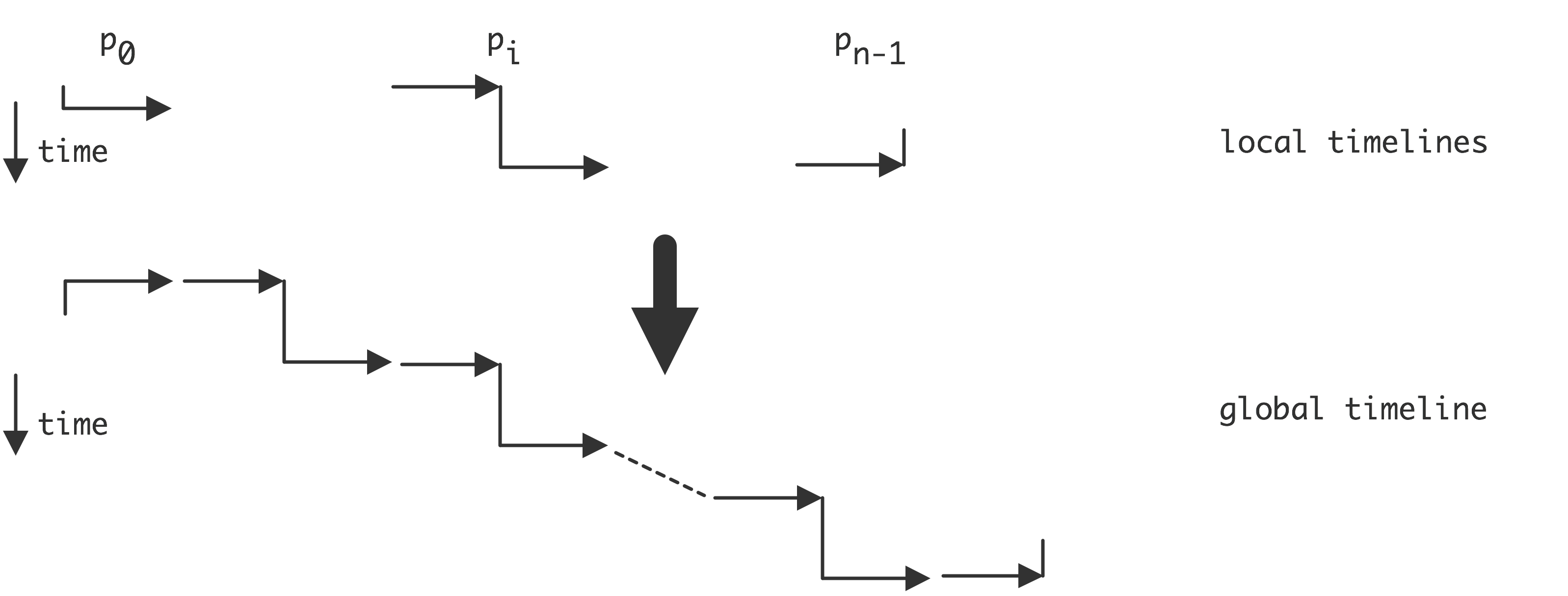\caption{Local and resulting global view of an algorithm for sending data to the right.}

the local timelines depicting the local processor code, and the resulting global behavior. You see that the processors are not working at the same time: we get serialized execution  .

What if we reverse the send and receive operations?

• If I am not the last processor, send my $x$ element to the right;
• If I am not the first processor, receive an $x$ element from the left and add it to my $y$ element.

This is illustrated in figure  2.6.3.1 and you see that

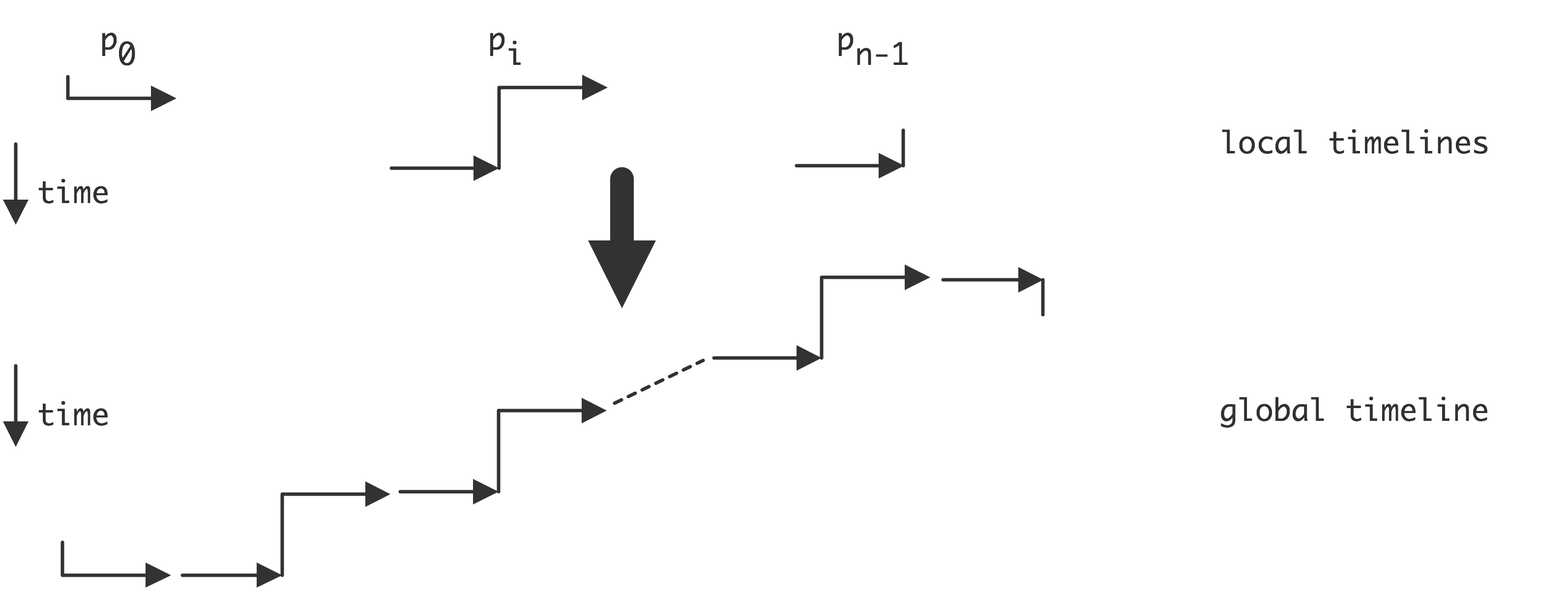\caption{Local and resulting global view of an algorithm for sending data to the right.}

again we get a serialized execution, except that now the processors are activated right to left.

If the algorithm in equation  2.6.3.1 had been cyclic: \begin{equation} \begin{cases} y_i\leftarrow y_i+x_{i-1}&i=1… n-1\\ y_0\leftarrow y_0+x_{n-1}&i=0 \end{cases} \label{eq:cyclic-add} \end{equation} the problem would be even worse. Now the last processor can not start its receive since it is blocked sending $x_{n-1}$ to processor 0. This situation, where the program can not progress because every processor is waiting for another, is called deadlock  .

The solution to getting an efficient code is to make as much of the communication happen simultaneously as possible. After all, there are no serial dependencies in the algorithm. Thus we program the algorithm as follows:

• If I am an odd numbered processor, I send first, then receive;
• If I am an even numbered processor, I receive first, then send.

This is illustrated in figure  2.6.3.1  , and we see that

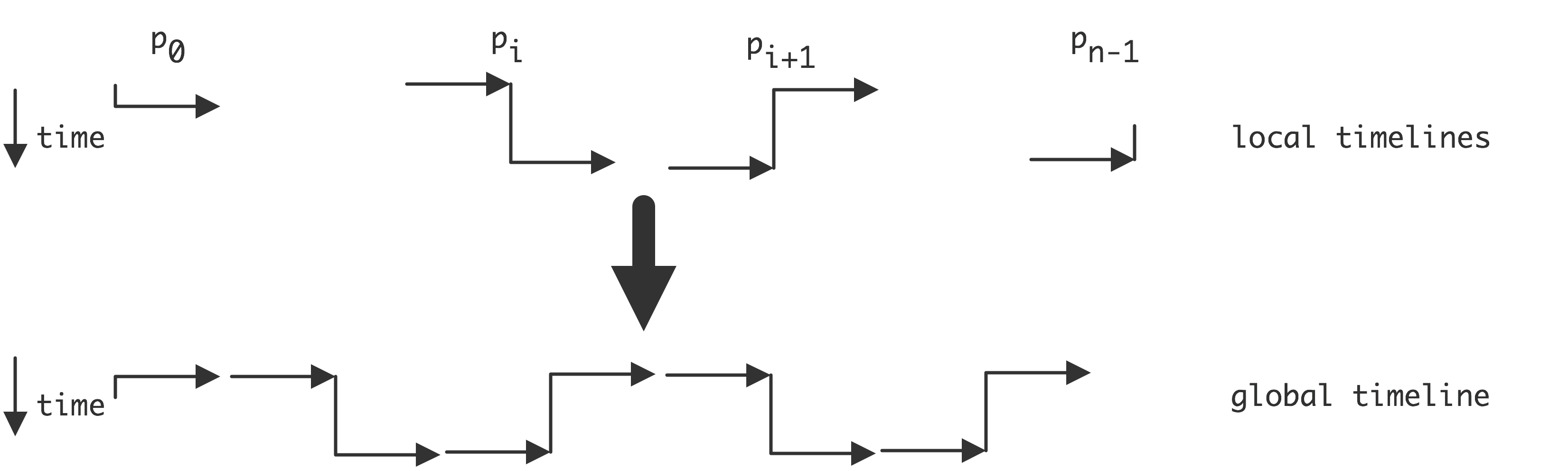\caption{Local and resulting global view of an algorithm for sending data to the right.}

the execution is now parallel.

Exercise Take another look at figure  2.3 of a parallel reduction. The basic actions are:

• receive data from a neighbor
• add it to your own data
• send the result on.

As you see in the diagram, there is at least one processor who does not send data on, and others may do a variable number of receives before they send their result on.

Write node code so that an SPMD program realizes the distributed reduction. Hint: write each processor number in binary. The algorithm uses a number of steps that is equal to the length of this bitstring.

• Assuming that a processor receives a message, express the distance to the origin of that message in the step number.
• Every processor sends at most one message. Express the step where this happens in terms of the binary processor number.

End of exercise

2.6.3.2 Blocking and non-blocking communication

crumb trail: > parallel > Parallel programming > Distributed memory programming through message passing > Blocking and non-blocking communication

The reason for blocking instructions is to prevent accumulation of data in the network. If a send instruction were to complete before the corresponding receive started, the network would have to store the data somewhere in the mean time. Consider a simple example:

buffer = ... ;  // generate some data
send(buffer,0); // send to processor 0
buffer = ... ;  // generate more data
send(buffer,1); // send to processor 1

After the first send, we start overwriting the buffer. If the data in it hasn't been received, the first set of values would have to be buffered somewhere in the network, which is not realistic. By having the send operation block, the data stays in the sender's buffer until it is guaranteed to have been copied to the recipient's buffer.

One way out of the problem of sequentialization or deadlock that arises from blocking instruction is the use of non-blocking communication instructions, which include explicit buffers for the data. With non-blocking send instruction, the user needs to allocate a buffer for each send, and check when it is safe to overwrite the buffer.

buffer0 = ... ;   // data for processor 0
send(buffer0,0);  // send to processor 0
buffer1 = ... ;   // data for processor 1
send(buffer1,1);  // send to processor 1
 ...
// wait for completion of all send operations.

2.6.3.3 The MPI library

crumb trail: > parallel > Parallel programming > Distributed memory programming through message passing > The MPI library

If OpenMP is the way to program shared memory, MPI   [mpi-reference] is the standard solution for programming distributed memory. MPI (`Message Passing Interface') is a specification for a library interface for moving data between processes that do not otherwise share data. The MPI routines can be divided roughly in the following categories:

• Process management. This includes querying the parallel environment and constructing subsets of processors.
• Point-to-point communication \index{point-to-point communication}. This is a set of calls where two processes interact. These are mostly variants of the send and receive calls.
• Collective calls. In these routines, all processors (or the whole of a specified subset) are involved. Examples are the broadcast call, where one processor shares its data with every other processor, or the gather call, where one processor collects data from all participating processors.

Let us consider how the OpenMP examples can be coded in MPI

(Note: {This is not a course in MPI programming, and consequently the examples will leave out many details of the MPI calls. If you want to learn MPI programming, consult for instance  [Gropp:UsingMPI1,Gropp:UsingMPI2,Gropp:UsingAdvancedMPI]  .}  )

. First of all, we no longer allocate

double a[ProblemSize];

but

double a[LocalProblemSize];

where the local size is roughly a $1/P$ fraction of the global size. (Practical considerations dictate whether you want this distribution to be as evenly as possible, or rather biased in some way.)

The parallel loop is trivially parallel, with the only difference that it now operates on a fraction of the arrays:

for (i=0; i<LocalProblemSize; i++) {
  a[i] = b[i];
}

However, if the loop involves a calculation based on the iteration number, we need to map that to the global value:

for (i=0; i<LocalProblemSize; i++) {
  a[i] = b[i]+f(i+MyFirstVariable);
}

(We will assume that each process has somehow calculated the values of LocalProblemSize and MyFirstVariable  .) Local variables are now automatically local, because each process has its own instance:

for (i=0; i<LocalProblemSize; i++) {
  t = b[i]*b[i];
  a[i] = sin(t) + cos(t);
}

However, shared variables are harder to implement. Since each process has its own data, the local accumulation has to be explicitly assembled:

for (i=0; i<LocalProblemSize; i++) {
  s = s + a[i]*b[i];
}
MPI_Allreduce(s,globals,1,MPI_DOUBLE,MPI_SUM);

The `reduce' operation sums together all local values  s into a variable globals that receives an identical value on each processor. This is known as a collective operation  .

Let us make the example slightly more complicated:

for (i=0; i<ProblemSize; i++) {
  if (i==0)
    a[i] = (b[i]+b[i+1])/2
  else if (i==ProblemSize-1)
    a[i] = (b[i]+b[i-1])/2
  else
    a[i] = (b[i]+b[i-1]+b[i+1])/3
}

If we had shared memory, we could write the following parallel code:

for (i=0; i<LocalProblemSize; i++) {
  bleft = b[i-1]; bright = b[i+1];
  a[i] = (b[i]+bleft+bright)/3
}

To turn this into valid distributed memory code, first we account for the fact that bleft and bright need to be obtained from a different processor for i==0 ( bleft  ), and for i==LocalProblemSize-1 ( bright  ). We do this with a exchange operation with our left and right neighbor processor:

// get bfromleft and bfromright from neighbor processors, then
for (i=0; i<LocalProblemSize; i++) {
  if (i==0) bleft=bfromleft;
    else bleft = b[i-1]
  if (i==LocalProblemSize-1) bright=bfromright;
    else bright = b[i+1];
  a[i] = (b[i]+bleft+bright)/3
}

Obtaining the neighbor values is done as follows. First we need to ask our processor number, so that we can start a communication with the processor with a number one higher and lower.

MPI_Comm_rank(MPI_COMM_WORLD,&myTaskID);
MPI_Sendrecv
   (/* to be sent:  */ &b[LocalProblemSize-1],
    /* destination  */ myTaskID+1,
    /* to be recvd: */ &bfromleft,
    /* source:      */ myTaskID-1, 
    /* some parameters omitted */ 
   );
MPI_Sendrecv(&b[0],myTaskID-1,
    &bfromright, /* ... */ );

There are still two problems with this code. First, the sendrecv operations need exceptions for the first and last processors. This can be done elegantly as follows:

MPI_Comm_rank(MPI_COMM_WORLD,&myTaskID);
MPI_Comm_size(MPI_COMM_WORLD,&nTasks);
if (myTaskID==0) leftproc = MPI_PROC_NULL;
  else leftproc = myTaskID-1;
if (myTaskID==nTasks-1) rightproc = MPI_PROC_NULL;
  else rightproc = myTaskID+1;
MPI_Sendrecv( &b[LocalProblemSize-1], &bfromleft,  rightproc );
MPI_Sendrecv( &b[0],                  &bfromright, leftproc);

Exercise There is still a problem left with this code: the boundary conditions from the original, global, version have not been taken into account. Give code that solves that problem.
End of exercise

MPI gets complicated if different processes need to take different actions, for example, if one needs to send data to another. The problem here is that each process executes the same executable, so it needs to contain both the send and the receive instruction, to be executed depending on what the rank of the process is.

if (myTaskID==0) {
  MPI_Send(myInfo,1,MPI_INT,/* to: */ 1,/* labeled: */,0,
    MPI_COMM_WORLD);
} else {
  MPI_Recv(myInfo,1,MPI_INT,/* from: */ 0,/* labeled: */,0,
    /* not explained here: */&status,MPI_COMM_WORLD);
}   

2.6.3.4 Blocking

crumb trail: > parallel > Parallel programming > Distributed memory programming through message passing > Blocking

Although MPI is sometimes called the `assembly language of parallel programming', for its perceived difficulty and level of explicitness, it is not all that hard to learn, as evinced by the large number of scientific codes that use it. The main issues that make MPI somewhat intricate to use are buffer management and blocking semantics.

These issues are related, and stem from the fact that, ideally, data should not be in two places at the same time. Let us briefly consider what happens if processor 1 sends data to processor 2. The safest strategy is for processor 1 to execute the send instruction, and then wait until processor 2 acknowledges that the data was successfully received. This means that processor 1 is temporarily blocked until processor 2 actually executes its receive instruction, and the data has made its way through the network. This is the standard behavior of the MPI_Send and MPI_Recv calls, which are said to use blocking communication  .

Alternatively, processor 1 could put its data in a buffer, tell the system to make sure that it gets sent at some point, and later checks to see that the buffer is safe to reuse. This second strategy is called non-blocking communication  , and it requires the use of a temporary buffer.

2.6.3.5 Collective operations

crumb trail: > parallel > Parallel programming > Distributed memory programming through message passing > Collective operations

In the above examples, you saw the MPI_Allreduce call, which computed a global sum and left the result on each processor. There is also a local version MPI_Reduce which computes the result only on operations} or collectives. The collectives are:

• [reduction]: each processor has a data item, and these items need to be combined arithmetically with an addition, multiplication, max, or min operation. The result can be left on one processor, or on all, in which case we call this an {\bf allreduce} operation.
• [broadcast]: one processor has a data item that all processors need to receive.
• [gather]: each processor has a data item, and these items need to be collected in an array, without combining them in an operations such as an addition. The result can be left on one processor, or on all, in which case we call this an {\bf allgather}.
• [scatter]: one processor has an array of data items, and each processor receives one element of that array.
• [all-to-all]: each processor has an array of items, to be scattered to all other processors.

Collective operations are blocking (see section  2.6.3.4  ), although MPI 3.0 (which is currently only a draft) will have non-blocking collectives. We will analyze the cost of collective operations in detail in section  6.1  .

2.6.3.6 Non-blocking communication

crumb trail: > parallel > Parallel programming > Distributed memory programming through message passing > Non-blocking communication

In a simple computer program, each instruction takes some time to execute, in a way that depends on what goes on in the processor. In parallel programs the situation is more complicated. A send operation, in its simplest form, declares that a certain buffer of data needs to be sent, and program execution will then stop until that buffer has been safely sent and received by another processor. This sort of operation is called a non-local operation since it depends on the actions of other processes, and a \indexterm{blocking communication} operation since execution will halt until a certain event takes place.

Blocking operations have the disadvantage that they can lead to deadlock  . In the context of message passing this describes the situation that a process is waiting for an event that never happens; for instance, it can be waiting to receive a message and the sender of that message is waiting for something else. Deadlock occurs if two processes are waiting for each other, or more generally, if you have a cycle of processes where each is waiting for the next process in the cycle. Example:

if ( /* this is process 0 */ )
   // wait for message from 1
else if ( /* this is process 1 */ )
   // wait for message from 0

A block receive here leads to deadlock. Even without deadlock, they can lead to considerable \indexterm{idle time} in the processors, as they wait without performing any useful work. On the other hand, they have the advantage that it is clear when the buffer can be reused: after the operation completes, there is a guarantee that the data has been safely received at the other end.

The blocking behavior can be avoided, at the cost of complicating the buffer semantics, by using non-blocking communication operations. A non-blocking send ( MPI_Isend  ) declares that a data buffer needs to be sent, but then does not wait for the completion of the corresponding receive. There is a second operation MPI_Wait that will actually block until the receive has been completed. The advantage of this decoupling of sending and blocking is that it now becomes possible to write:

MPI_ISend(somebuffer,&handle); // start sending, and
    // get a handle to this particular communication
{ ... }  // do useful work on local data
MPI_Wait(handle); // block until the communication is completed;
{ ... }  // do useful work on incoming data

With a little luck, the local operations take more time than the communication, and you have completely eliminated the communication time.

In addition to non-blocking sends, there are non-blocking receives. A typical piece of code then looks like

MPI_ISend(sendbuffer,&sendhandle);
MPI_IReceive(recvbuffer,&recvhandle);
{ ... }  // do useful work on local data
MPI_Wait(sendhandle); Wait(recvhandle);
{ ... }  // do useful work on incoming data

Exercise 2.6.3.1 solves the problem using non-blocking sends and receives. What is the disadvantage of this code over a blocking solution?
End of exercise

2.6.3.7 MPI version 1 and 2 and 3

crumb trail: > parallel > Parallel programming > Distributed memory programming through message passing > MPI version 1 and 2 and 3

The first MPI standard  [mpi-ref] had a number of notable omissions, which are included in the MPI 2 standard  [mpi-2-reference]  . One of these concerned parallel input/output: there was no facility for multiple processes to access the same file, even if the underlying hardware would allow that. A separate project MPI-I/O has now been rolled into the MPI-2 standard. We will discuss parallel I/O in this book.

A second facility missing in MPI, though it was present in PVM   [pvm-1,pvm-2] which predates MPI, is process management: there is no way to create new processes and have them be part of the parallel run.

Finally, MPI-2 has support for one-sided communication: one process puts data into the memory of another, without the receiving process doing an actual receive instruction. We will have a short discussion in section  2.6.3.8 below.

With MPI-3 the standard has gained a number of new features, such as non-blocking collectives, neighborhood collectives, and a profiling interface. The one-sided mechanisms have also been updated.

2.6.3.8 One-sided communication

crumb trail: > parallel > Parallel programming > Distributed memory programming through message passing > One-sided communication

The MPI way of writing matching send and receive instructions is not ideal for a number of reasons. First of all, it requires the programmer to give the same data description twice, once in the send and once in the receive call. Secondly, it requires a rather precise orchestration of communication if deadlock is to be avoided; the alternative of using asynchronous calls is tedious to program, requiring the program to manage a lot of buffers. Lastly, it requires a receiving processor to know how many incoming messages to expect, which can be tricky in irregular applications. Life would be so much easier if it was possible to pull data from another processor, or conversely to put it on another processor, without that other processor being explicitly involved.

This style of programming is further encouraged by the existence of RDMA support on some hardware. An early example was the Cray T3E  . These days, one-sided communication is widely available through its incorporation in the MPI-2 library; section  2.6.3.7  .

Let us take a brief look at one-sided communication in MPI-2, using averaging of array values as an example: \begin{equation} \forall_i\colon a_i\leftarrow (a_i+a_{i-1}+a_{i+1})/3. \end{equation} The MPI parallel code will look like

// do data transfer
a_local = (a_local+left+right)/3

It is clear what the transfer has to accomplish: the a_local variable needs to become the left variable on the processor with the next higher rank, and the right variable on the one with the next lower rank.

First of all, processors need to declare explicitly what memory area is available for one-sided transfer, the so-called `window'. In this example, that consists of the a_local  , left  , and right variables on the processors:

MPI_Win_create(&a_local,...,&data_window);
MPI_Win_create(&left,....,&left_window);
MPI_Win_create(&right,....,&right_window);

The code now has two options: it is possible to push data out

target = my_tid-1;
MPI_Put(&a_local,...,target,right_window);
target = my_tid+1;
MPI_Put(&a_local,...,target,left_window);

or to pull it in

data_window = a_local;
source = my_tid-1;
MPI_Get(&right,...,data_window);
source = my_tid+1;
MPI_Get(&left,...,data_window);

The above code will have the right semantics if the Put and Get calls are blocking; see section  2.6.3.4  . However, part of the attraction of one-sided communication is that it makes it easier to express communication, and for this, a non-blocking semantics is assumed.

The problem with non-blocking one-sided calls is that it becomes necessary to ensure explicitly that communication is successfully completed. For instance, if one processor does a one-sided put operation on another, the other processor has no way of checking that the data has arrived, or indeed that transfer has begun at all. Therefore it is necessary to insert a global barrier in the program, for which every package has its own implementation. In MPI-2 the relevant call is the MPI_Win_fence routine. These barriers in effect divide the program execution in supersteps ; see section  2.6.8  .

Another form of one-sided communication is used in the Charm++ package; see section  2.6.7  .

2.6.4 Hybrid shared/distributed memory computing

crumb trail: > parallel > Parallel programming > Hybrid shared/distributed memory computing

Modern architectures are often a mix of shared and distributed memory. For instance, a cluster will be distributed on the level of the nodes, but sockets and cores on a node will have shared memory. One level up, each socket can have a shared L3 cache but separate L2 and L1 caches. Intuitively it seems clear that a mix of shared and distributed programming techniques would give code that is optimally matched to the architecture. In this section we will discuss such hybrid programming models, and discuss their efficacy.

A common setup of clusters uses distributed memory nodes sockets using MPI to communicate between the nodes ( inter-node communication  ) and OpenMP for parallelism on the node ( intra-node communication  ).

In practice this is realized as follows:

• On each node a single MPI process is started (rather than one per core);
• This one MPI process then uses OpenMP (or another threading protocol) to spawn as many threads are there are independent sockets or cores on the node.
• The OpenMP threads can then access the shared memory of the node.

The alternative would be to have an MPI process on each core or socket and do all communication through message passing, even between processes that can see the same shared memory.

Remark For reasons of affinity it may be desirable to start one MPI process per socket, rather than per node. This does not materially alter the above argument.
End of remark

This hybrid strategy may sound like a good idea but the truth is complicated.

• Message passing between MPI processes sounds like it's more expensive than communicating through shared memory. However, optimized versions of MPI can typically detect when processes are on the same node, and they will replace the message passing by a simple data copy. The only argument against using MPI is then that each process has its own data space, so there is memory overhead because each process has to allocate space for buffers and duplicates of the data that is copied.
• Threading is more flexible: if a certain part of the code needs more memory per process, an OpenMP approach could limit the number of threads on that part. On the other hand, flexible handling of threads incurs a certain amount of OS overhead that MPI does not have with its fixed processes.
• Shared memory programming is conceptually simple, but there can be unexpected performance pitfalls. For instance, the performance of two processes can now be impeded by the need for maintaining cache coherence and by false sharing  .

On the other hand, the hybrid approach offers some advantage since it bundles messages. For instance, if two MPI processes on one node send messages to each of two processes on another node there would be four messages; in the hybrid model these would be bundled into one message.

Exercise Analyze the discussion in the last item above. Assume that the bandwidth between the two nodes is only enough to sustain one message at a time. What is the cost savings of the hybrid model over the purely distributed model? Hint: consider bandwidth and latency separately.
End of exercise

This bundling of MPI processes may have an advantage for a deeper technical reason. In order to support a handshake protocol  , each MPI process needs a small amount of buffer space for each other process. With a larger number of processes this can be a limitation, so bundling is attractive on high core count processors such as the Intel Xeon Phi  .

The MPI library is explicit about what sort of threading it supports: you can query whether multi-threading is supported at all, whether all MPI calls have to originate from one thread or one thread at-a-time, or whether there is complete freedom in making MPI calls from threads.

2.6.5 Parallel languages

crumb trail: > parallel > Parallel programming > Parallel languages

One approach to mitigating the difficulty of parallel programming is the design of languages that offer explicit support for parallelism. There are several approaches, and we will see some examples.

• Some languages reflect the fact that many operations in scientific computing are data parallel (section  2.5.1  ). Languages such as HPF (section  2.6.5.3  ) have an array syntax  , where operations such as addition of arrays can be expressed as A = B+C  . This syntax simplifies programming, but more importantly, it specifies operations at an abstract level, so that a lower level can make specific decision about how to handle parallelism. However, the data parallelism expressed in HPF is only of the simplest sort, where the data are contained in regular arrays. Irregular data parallelism is harder; the Chapel language (section  2.6.5.5  ) makes an attempt at addressing this.
• Another concept in parallel languages, not necessarily orthogonal to the previous, is that of PGAS model: there is only one address space (unlike in the MPI model), but this address space is partitioned, and each partition has affinity with a thread or process. Thus, this model encompasses both SMP and distributed shared memory. A typical PGAS language, UPC  , allows you to write programs that for the most part looks like regular C code. However, by indicating how the major arrays are distributed over processors, the program can be executed in parallel.

2.6.5.1 Discussion

crumb trail: > parallel > Parallel programming > Parallel languages > Discussion

Parallel languages hold the promise of making parallel programming easier, since they make communication operations appear as simple copies or arithmetic operations. However, by doing so they invite the user to write code that may not be efficient, for instance by inducing many small messages.

FIGURE 2.14: Data shift that requires communication.

As an example, consider arrays a,b that have been horizontally partitioned over the processors, and that are shifted (see figure  2.14  ):

for (i=0; i<N; i++)
  for (j=0; j<N/np; j++)
    a[i][j+joffset] = b[i][j+1+joffset]

If this code is executed on a shared memory machine, it will be efficient, but a naive translation in the distributed case will have a single number being communicated in each iteration of the i  loop. Clearly, these can be combined in a single buffer send/receive operation, but compilers are usually unable to make this transformation. As a result, the user is forced to, in effect, re-implement the blocking that needs to be done in an MPI implementation:

for (i=0; i<N; i++)
  t[i] = b[i][N/np+joffset]
for (i=0; i<N; i++)
  for (j=0; j<N/np-1; j++) {
    a[i][j] = b[i][j+1]
    a[i][N/np] = t[i]
  }

On the other hand, certain machines support direct memory copies through global memory hardware. In that case, PGAS languages can be more efficient than explicit message passing, even with physically distributed memory.

2.6.5.2 Unified Parallel C

crumb trail: > parallel > Parallel programming > Parallel languages > Unified Parallel C

UPC   [UPC:homepage] is an extension to the C language. Its main source of parallelism is data parallelism  , where the compiler discovers independence of operations on arrays, and assigns them to separate processors. The language has an extended array declaration, which allows the user to specify whether the array is partitioned by blocks, or in a round-robin fashion.

The following program in UPC performs a vector-vector addition.

//vect_add.c
#include <upc_relaxed.h>
#define N 100*THREADS
shared int v1[N], v2[N], v1plusv2[N];
void main() {
  int i;
  for(i=MYTHREAD; i<N; i+=THREADS)
    v1plusv2[i]=v1[i]+v2[i];
}

The same program with an explicitly parallel loop construct:

//vect_add.c
#include <upc_relaxed.h>
#define N 100*THREADS
shared int v1[N], v2[N], v1plusv2[N];
void main()
{
  int i;
  upc_forall(i=0; i<N; i++; i)
    v1plusv2[i]=v1[i]+v2[i];
}

is comparable to UPC in spirit, but based on Java rather than on C.

2.6.5.3 High Performance Fortran

crumb trail: > parallel > Parallel programming > Parallel languages > High Performance Fortran

High Performance Fortran

(Note: {This section quoted from Wikipedia}  )

(HPF) is an extension of Fortran 90 with constructs that support parallel computing, published by the High Performance Fortran Forum (HPFF). The HPFF was convened and chaired by Ken Kennedy of Rice University. The first version of the HPF Report was published in 1993.

Building on the array syntax introduced in Fortran 90, HPF uses a data parallel model of computation to support spreading the work of a single array computation over multiple processors. This allows efficient implementation on both SIMD and MIMD style architectures. HPF features included:

• New Fortran statements, such as FORALL, and the ability to create PURE (side effect free) procedures;
• The use of compiler directives for recommended distributions of array data;
• Extrinsic procedure interface for interfacing to non-HPF parallel procedures such as those using message passing;
• Additional library routines, including environmental inquiry, parallel prefix/suffix (e.g., 'scan'), data scattering, and sorting operations.

Fortran 95 incorporated several HPF capabilities. While some vendors did incorporate HPF into their compilers in the 1990s, some aspects proved difficult to implement and of questionable use. Since then, most vendors and users have moved to OpenMP-based parallel processing. However, HPF continues to have influence. For example the proposed BIT data type for the upcoming Fortran-2008 standard contains a number of new intrinsic functions taken directly from HPF.

2.6.5.4 Co-array Fortran

crumb trail: > parallel > Parallel programming > Parallel languages > Co-array Fortran

CAF is an extension to the Fortran 95/2003 language. The main mechanism to support parallelism is an extension to the array declaration syntax, where an extra dimension indicates the parallel distribution. For instance, in

Real,dimension(100),codimension[*] :: X
Real :: Y(100)[*]
Real :: Z(100,200)[10,0:9,*]

arrays X,Y have 100 elements on each processor. Array Z behaves as if the available processors are on a three-dimensional grid, with two sides specified and the third adjustable to accommodate the available processors.

Communication between processors is now done through copies along the (co-)dimensions that describe the processor grid.

The Fortran 2008 standard includes co-arrays.

2.6.5.5 Chapel

crumb trail: > parallel > Parallel programming > Parallel languages > Chapel

Chapel  [Chapel:homepage] is a new parallel programming language

(Note: {This section quoted from the Chapel homepage.}  )

being developed by Cray Inc. as part of the DARPA-led High Productivity Computing Systems program (HPCS). Chapel is designed to improve the productivity of high-end computer users while also serving as a portable parallel programming model that can be used on commodity clusters or desktop multicore systems. Chapel strives to vastly improve the programmability of large-scale parallel computers while matching or beating the performance and portability of current programming models like MPI.

Chapel supports a multithreaded execution model via high-level abstractions for data parallelism, task parallelism, concurrency, and nested parallelism. Chapel's locale type enables users to specify and reason about the placement of data and tasks on a target architecture in order to tune for locality. Chapel supports global-view data aggregates with user-defined implementations, permitting operations on distributed data structures to be expressed in a natural manner. In contrast to many previous higher-level parallel languages, Chapel is designed around a multiresolution philosophy, permitting users to initially write very abstract code and then incrementally add more detail until they are as close to the machine as their needs require. Chapel supports code reuse and rapid prototyping via object-oriented design, type inference, and features for generic programming.

Chapel was designed from first principles rather than by extending an existing language. It is an imperative block-structured language, designed to be easy to learn for users of C, C++, Fortran, Java, Perl, Matlab, and other popular languages. While Chapel builds on concepts and syntax from many previous languages, its parallel features are most directly influenced by ZPL, High-Performance Fortran (HPF), and the Cray MTA's extensions to C and Fortran.

Here is vector-vector addition in Chapel:

const BlockDist= newBlock1D(bbox=[1..m], tasksPerLocale=...);
const ProblemSpace: domain(1, 64)) distributed BlockDist = [1..m];
var A, B, C: [ProblemSpace] real;
forall(a, b, c) in(A, B, C) do
  a = b + alpha * c;

2.6.5.6 Fortress

crumb trail: > parallel > Parallel programming > Parallel languages > Fortress

Fortress  [Fortress:homepage] is a programming language developed by Sun Microsystems. Fortress

(Note: {This section quoted from the Fortress homepage.}  )

aims to make parallelism more tractable in several ways. First, parallelism is the default. This is intended to push tool design, library design, and programmer skills in the direction of parallelism. Second, the language is designed to be more friendly to parallelism. Side-effects are discouraged because side-effects require synchronization to avoid bugs. Fortress provides transactions, so that programmers are not faced with the task of determining lock orders, or tuning their locking code so that there is enough for correctness, but not so much that performance is impeded. The Fortress looping constructions, together with the library, turns "iteration" inside out; instead of the loop specifying how the data is accessed, the data structures specify how the loop is run, and aggregate data structures are designed to break into large parts that can be effectively scheduled for parallel execution. Fortress also includes features from other languages intended to generally help productivity -- test code and methods, tied to the code under test; contracts that can optionally be checked when the code is run; and properties, that might be too expensive to run, but can be fed to a theorem prover or model checker. In addition, Fortress includes safe-language features like checked array bounds, type checking, and garbage collection that have been proven-useful in Java. Fortress syntax is designed to resemble mathematical syntax as much as possible, so that anyone solving a problem with math in its specification can write a program that is visibly related to its original specification.

2.6.5.7 X10

crumb trail: > parallel > Parallel programming > Parallel languages > X10

X10 is an experimental new language currently under development at IBM in collaboration with academic partners. The X10 effort is part of the IBM PERCS project (Productive Easy-to-use Reliable Computer Systems) in the DARPA program on High Productivity Computer Systems. The PERCS project is focused on a hardware-software co-design methodology to integrate advances in chip technology, architecture, operating systems, compilers, programming language and programming tools to deliver new adaptable, scalable systems that will provide an order-of-magnitude improvement in development productivity for parallel applications by 2010.

X10 aims to contribute to this productivity improvement by developing a new programming model, combined with a new set of tools integrated into Eclipse and new implementation techniques for delivering optimized scalable parallelism in a managed runtime environment. X10 is a type-safe, modern, parallel, distributed object-oriented language intended to be accessible to Java(TM) programmers. It is targeted to future low-end and high-end systems with nodes that are built out of multi-core SMP chips with non-uniform memory hierarchies, and interconnected in scalable cluster configurations. A member of the Partitioned Global Address Space (PGAS) family of languages, X10 highlights the explicit reification of locality in the form of places; lightweight activities embodied in async, future, foreach, and ateach constructs; constructs for termination detection (finish) and phased computation (clocks); the use of lock-free synchronization (atomic blocks); and the manipulation of global arrays and data structures.

2.6.5.8 Linda

crumb trail: > parallel > Parallel programming > Parallel languages > Linda

As should be clear by now, the treatment of data is by far the most important aspect of parallel programming, far more important than algorithmic considerations. The programming system Linda   [Gelernter85generativecommunication,Linda-CACM]  , also called a coordination language  , is designed to address the data handling explicitly. Linda is not a language as such, but can, and has been, incorporated into other languages.

The basic concept of Linda is the tuple space : data is added to a pool of globally accessible information by adding a label to it. Processes then retrieve data by the label value, and without needing to know which processes added the data to the tuple space.

Linda is aimed primarily at a different computation model than is relevant for HPC : it addresses the needs of asynchronous communicating processes. However, is has been used for scientific computation  [Deshpande92efficientparallel]  . For instance, in parallel simulations of the heat equation (section  4.3  ), processors can write their data into tuple space, and neighboring processes can retrieve their \indexterm{ghost region} without having to know its provenance. Thus, Linda becomes one way of implementing one-sided communication  .

2.6.5.9 The Global Arrays library

crumb trail: > parallel > Parallel programming > Parallel languages > The Global Arrays library

The Global Arrays library ( http://www.emsl.pnl.gov/docs/global/  ) is another example of one-sided communication  , and in fact it predates MPI. This library has as its prime data structure Cartesian product arrays

(Note: {This means that if the array is three-dimensional, it can be described by three integers $n_1,n_2,n_3$, and each point has a coordinate $(i_1,i_2,i_3)$ with $1\leq i_1\leq n_1$ et cetera.}  )

 , distributed over a processor grid of the same or lower dimension. Through library calls, any processor can access any sub-brick out of the array in either a put or get operation. These operations are non-collective. As with any one-sided protocol, a barrier sync is necessary to ensure completion of the sends/receives.

2.6.6 OS-based approaches

crumb trail: > parallel > Parallel programming > OS-based approaches

It is possible to design an architecture with a shared address space, and let the data movement be handled by the operating system. The Kendall Square computer  [KSRallcache] had an architecture name `all-cache', where no data was directly associated with any processor. Instead, all data was considered to be cached on a processor, and moved through the network on demand, much like data is moved from main memory to cache in a regular CPU. This idea is analogous to the NUMA support in current SGI architectures.

2.6.7 Active messages

crumb trail: > parallel > Parallel programming > Active messages

The MPI paradigm (section  2.6.3.3  ) is traditionally based on two-sided operations: each data transfer requires an explicit send and receive operation. This approach works well with relatively simple codes, but for complicated problems it becomes hard to orchestrate all the data movement. One of the ways to simplify consists of using active messages  . This is used in the package Charm++ [charmpp]  .

With active messages, one processor can send data to another, without that second processor doing an explicit receive operation. Instead, the recipient declares code that handles the incoming data, a `method' in objective orientation parlance, and the sending processor calls this method with the data that it wants to send. Since the sending processor in effect activates code on the other processor, this is also known as remote method invocation  . A big advantage of this method is that overlap of communication and computation becomes easier to realize.

As an example, consider the matrix-vector multiplication with a tridiagonal matrix \begin{equation} \forall_i\colon y_i\leftarrow 2x_i-x_{i+1}-x_{i-1}. \end{equation} See section  4.2.2 for an explanation of the origin of this problem in PDEs  . Assuming that each processor has exactly one index $i$, the MPI code could look like:

if ( /* I am the first or last processor */ )
   n_neighbors = 1;
else
   n_neighbors = 2;

/* do the MPI_Isend operations on my local data */

sum = 2*local_x_data;
received = 0;
for (neighbor=0; neighbor<n_neighbors; neighbor++) {
   MPI_WaitAny( /* wait for any incoming data */ )
   sum = sum - /* the element just received */
   received++
   if (received==n_neighbors)
      local_y_data = sum
}

With active messages this looks like

void incorporate_neighbor_data(x) {
   sum = sum-x;
   if (received==n_neighbors)
      local_y_data = sum
}
sum = 2*local_xdata;
received = 0;
all_processors[myid+1].incorporate_neighbor_data(local_x_data);
all_processors[myid-1].incorporate_neighbor_data(local_x_data);

2.6.8 Bulk synchronous parallelism

crumb trail: > parallel > Parallel programming > Bulk synchronous parallelism

The MPI library (section  2.6.3.3  ) can lead to very efficient code. The price for this is that the programmer needs to spell out the communication in great detail. On the other end of the spectrum, PGAS languages (section  2.6.5  ) ask very little of the programmer, but give not much performance in return. One attempt to find a middle ground is the BSP model  [Valiant:1990:BSP,Skillicorn96questionsand]  . Here the programmer needs to spell out the communications, but not their ordering.

The BSP model orders the program into a sequence of supersteps  , each of which ends with a barrier synchronization. The communications that are started in one superstep are all asynchronous and rely on the barrier for their completion. This makes programming easier and removes the possibility of deadlock. Moreover, all communication are of the one-sided communication type.

Exercise Consider the parallel summing example in section  2.1  . Argue that a BSP implementation needs $\log_2n$ supersteps.
End of exercise

Because of its synchronization of the processors through the barriers concluding the supersteps the BSP model can do a simple cost analysis of parallel algorithms.

Another aspect of the BSP model is its use of overdecomposition of the problem, where multiple processes are assigned to each processor, as well as random placement of data and tasks. This is motivated with a statistical argument that shows it can remedy load imbalance  . If there are $p$ processors and if in a superstep $p$ remote accesses are made, with high likelihood some processor receives $\log p/\log \log p$ accesses, while others receive none. Thus, we have a load imbalance that worsens with increasing processor count. On the other hand, if $p\log p$ accesses are made, for instance because there are $\log p$ processes on each processor, the maximum number of accesses is $3\log p$ with high probability. This means the load balance is within a constant factor of perfect.

The BSP model is implemented in BSPlib  [BSPlib]  . Other system can be said to be BSP-like in that they use the concept of supersteps; for instance Google's Pregel   [Pregel:podc2009]  .

2.6.9 Data dependencies

crumb trail: > parallel > Parallel programming > Data dependencies

If two statements refer to the same data item, we say that there is a data dependency between the statements. Such dependencies limit the extent to which the execution of the statements can be rearranged. The study of this topic probably started in the 1960s, when processors could execute statements out of order to increase throughput. The re-ordering of statements was limited by the fact that the execution had to obey the program order semantics: the result had to be as if the statements were executed strictly in the order in which they appear in the program.

These issues of statement ordering, and therefore of data dependencies, arise in several ways:

• A parallelizing compiler has to analyze the source to determine what transformations are allowed;
• if you parallelize a sequential code with OpenMP directives, you have to perform such an analysis yourself.

Here are two types of activity that require such an analysis:

• When a loop is parallelized, the iterations are no longer executed in their program order, so we have to check for dependencies.
• The introduction of tasks also means that parts of a program can be executed in a different order from in which they appear in a sequential execution.

The easiest case of dependency analysis is that of detecting that loop iterations can be executed independently. Iterations are of course independent if a data item is read in two different iterations, but if the same item is read in one iteration and written in another, or written in two different iterations, we need to do further analysis.

Analysis of data dependencies can be performed by a compiler, but compilers take, of necessity, a conservative approach. This means that iterations may be independent, but can not be recognized as such by a compiler. Therefore, OpenMP shifts this responsibility to the programmer.

We will now discuss data depencies in some detail.

2.6.9.1 Types of data dependencies

crumb trail: > parallel > Parallel programming > Data dependencies > Types of data dependencies

The three types of dependencies are:

• flow dependencies, or `read-after-write';
• anti dependencies, or `write-after-read'; and
• output dependencies, or `write-after-write'.

These dependencies can be studied in scalar code, and in fact compilers do this to determine whether statements can be rearranged, but we will mostly be concerned with their appearance in loops, since in scientific computation much of the work appears there.

Flow dependencies

Flow dependencies are not a problem if the read and write occur in the same loop iteration:

for (i=0; i<N; i++) {
  x[i] = .... ;
  .... = ... x[i] ... ;
}

On the other hand, if the read happens in a later iteration, there is no simple way to parallelize or vectorize the loop:

for (i=0; i<N; i++) {
  .... = ... x[i] ... ;
  x[i+1] = .... ;
}

This usually requires rewriting the code.

Exercise Consider the code

for (i=0; i<N; i++) {
  a[i] = f(x[i]);
  x[i+1] = g(b[i]);
}

where f() and g() denote arithmetical expressions with out further dependencies on x or  i  . Show that this loop can be parallelized/vectorized if you are allowed to use a temporary array.
End of exercise

\heading {Anti dependencies}

The simplest case of an anti dependency or write-after-read is a reduction:

for (i=0; i<N; i++) {
  t = t + .....
}

This can be dealt with by explicit declaring the loop to be a reduction, or to use any of the other strategies in section  6.1.2  .

If the read and write are on an array the situation is more complicated. The iterations in this fragment

for (i=0; i<N; i++) {
  x[i] = ... x[i+1] ... ;
}

can not be executed in arbitrary order as such. However, conceptually there is no dependency. We can solve this by introducing a temporary array:

for (i=0; i<N; i++)
  xtmp[i] = x[i];
for (i=0; i<N; i++) {
  x[i] = ... xtmp[i+1] ... ;
}

This is an example of a transformation that a compiler is unlikely to perform, since it can greatly affect the memory demands of the program. Thus, this is left to the programmer.

\heading {Output dependencies}

The case of an output dependency or write-after-write does not occur by itself: if a variable is written twice in sequence without an intervening read, the first write can be removed without changing the meaning of the program. Thus, this case reduces to a flow dependency.

Other output dependencies can also be removed. In the following code, t  can be declared private, thereby removing the dependency.

for (i=0; i<N; i++) {
  t = f(i)
  s += t*t;
}

If the final value of t is wanted, the lastprivate can be used in OpenMP.

2.6.9.2 Parallelizing nested loops

crumb trail: > parallel > Parallel programming > Data dependencies > Parallelizing nested loops

In the above examples, data dependencies were non-trivial if in iteration $i$ of a loop different indices appeared, such as $i$ and $i+1$. Conversely, loops such as

for (int i=0; i<N; i++)
  x[i] = x[i]+f(i);

are simple to parallelize. Nested loops, however, take more thought. OpenMP has a `collapse' directive for loops such as

for (int i=0; i<M; i++)
  for (int j=0; j<N; j++)
    x[i][j] = x[i][j] + y[i] + z[j];

Here, the whole $i,j$ iteration space is parallel.

How is that with:

for (n = 0; n < NN; n++)
  for (i = 0; i < N; i++)
    for (j = 0; j < N; j++)
      a[i] += B[i][j]*c[j] + d[n];

Exercise Do a reuse analysis on this loop. Assume that a,b,c do not all fit in cache together.

Now assume that c and one row of  b fit in cache, with a little room to spare. Can you find a loop interchange that will greatly benefit performance? Write a test to confirm this.
End of exercise

Analyzing this loop nest for parallelism, you see that the j -loop is a reduction, and the n -loop has flow dependencies: every a[i] is updated in every n -iteration. The conclusion is that you can only reasonable parallelize the i -loop.

Exercise How does this parallelism analysis relate to the loop exchange from exercise  2.6.9.2 ? Is the loop after exchange still parallelizable?

If you speak OpenMP, confirm your answer by writing code that adds up the elements of  a  . You should get the same answer no matter the exchanges and the introduction of OpenMP parallelism.
End of exercise

2.6.10 Program design for parallelism

crumb trail: > parallel > Parallel programming > Program design for parallelism

A long time ago it was thought that some magic combination of compiler and runtime system could transform an existing sequential program into a parallel one. That hope has long evaporated, so these days a parallel program will have been written from the ground up as parallel. Of course there are different types of parallelism, and they each have their own implications for precisely how you design your parallel program. In this section we will briefly look into some of the issues.

2.6.10.1 Parallel data structures

crumb trail: > parallel > Parallel programming > Program design for parallelism > Parallel data structures

One of the issues in parallel program design is the use of AOS vs SOA  . In normal program design you often define a structure

struct { int number; double xcoord,ycoord; } _Node;
struct { double xtrans,ytrans} _Vector;
typedef struct _Node* Node;
typedef struct _Vector* Vector;

and if you need a number of them you create an array of such structures.

Node *nodes = (Node*) malloc( n_nodes*sizeof(struct _Node) );

This is the AOS design.

Now suppose that you want to parallelize an operation

void shift(Node the_point,Vector by) {
  the_point->xcoord += by->xtrans;
  the_point->ycoord += by->ytrans;
}

which is done in a loop

for (i=0; i<n_nodes; i++) {
  shift(nodes[i],shift_vector);
}

This code has the right structure for MPI programming (section  2.6.3.3  ), where every processor has its own local array of nodes. This loop is also readily parallelizable with OpenMP (section  2.6.2  ).

However, in the 1980s codes had to be substantially rewritten as it was realized that the AOS design was not good for vector computers. In that case you operands need to be contiguous, and so codes had to go to a SOA design:

node_numbers = (int*) malloc( n_nodes*sizeof(int) );
node_xcoords = // et cetera
node_ycoords = // et cetera

and you would iterate

for (i=0; i<n_nodes; i++) {
  node_xoords[i] += shift_vector->xtrans;
  node_yoords[i] += shift_vector->ytrans;
}

Oh, did I just say that the original SOA design was best for distributed memory programming? That meant that 10 years after the vector computer era everyone had to rewrite their codes again for clusters. And of course nowadays, with increasing SIMD width  , we need to go part way back to the AOS design. (There is some experimental software support for this transformation in the Intel ispc project, http://ispc.github.io/  , which translates SPMD code to SIMD  .)

2.6.10.2 Latency hiding

crumb trail: > parallel > Parallel programming > Program design for parallelism > Latency hiding

Communication between processors is typically slow, slower than data transfer from memory on a single processor, and much slower than operating on data. For this reason, it is good to think about the relative volumes of network traffic versus `useful' operations when designing a parallel program. There has to be enough work per processor to offset the communication.

Another way of coping with the relative slowness of communication is to arrange the program so that the communication actually happens while some computation is going on. This is referred to as overlapping computation with communication or latency hiding  .

For example, consider the parallel execution of a matrix-vector product $y=Ax$ (there will be further discussion of this operation in section  6.2.1  ). Assume that the vectors are distributed, so each processor $p$ executes \begin{equation} \forall_{i\in I_p}\colon y_i=\sum_j a_{ij}x_j. \end{equation} Since $x$ is also distributed, we can write this as \begin{equation} \forall_{i\in I_p}\colon y_i= \left(\sum_{\mbox{\small $j$ local}} +\sum_{\mbox{\small $j$ not local}} \right) a_{ij}x_j. \end{equation} This scheme is illustrated in figure  2.6.10.2  .

\caption{The parallel matrix-vector product with a blockrow distribution.}

We can now proceed as follows:

• Start the transfer of non-local elements of $x$;
• Operate on the local elements of $x$ while data transfer is going on;
• Make sure that the transfers are finished;
• Operate on the non-local elements of $x$.

Exercise How much can you gain from overlapping computation and communication? Hint: consider the border cases where computation takes zero time and and there is only communication, and the reverse. Now consider the general case.
End of exercise

Of course, this scenario presupposes that there is software and hardware support for this overlap. MPI allows for this (see section  2.6.3.6  ), through so-called asynchronous communication or \indexterm{non-blocking communication} routines. This does not immediately imply that overlap will actually happen, since hardware support is an entirely separate question.

2.7 Topologies

crumb trail: > parallel > Topologies

If a number of processors are working together on a single task, most likely they need to communicate data. For this reason there needs to be a way for data to make it from any processor to any other. In this section we will discuss some of the possible schemes to connect the processors in a parallel machine. Such a scheme is called a (processor) topology  .

In order to get an appreciation for the fact that there is a genuine problem here, consider two simple schemes that do not `scale up':

• Ethernet is a connection scheme where all machines on a network are on a single cable (see remark below). If one machine puts a signal on the wire to send a message, and another also wants to send a message, the latter will detect that the sole available communication channel is occupied, and it will wait some time before retrying its send operation. Receiving data on ethernet is simple: messages contain the address of the intended recipient, so a processor only has to check whether the signal on the wire is intended for it.

  The problems with this scheme should be clear. The capacity of the communication channel is finite, so as more processors are connected to it, the capacity available to each will go down. Because of the scheme for resolving conflicts, the average delay before a message can be started will also increase.

• In a fully connected configuration, each processor has one wire for the communications with each other processor. This scheme is perfect in the sense that messages can be sent in the minimum amount of time, and two messages will never interfere with each other. The amount of data that can be sent from one processor is no longer a decreasing function of the number of processors; it is in fact an increasing function, and if the network controller can handle it, a processor can even engage in multiple simultaneous communications.

  The problem with this scheme is of course that the design of the network interface of a processor is no longer fixed: as more processors are added to the parallel machine, the network interface gets more connecting wires. The network controller similarly becomes more complicated, and the cost of the machine increases faster than linearly in the number of processors.

Remark The above description of Ethernet is of the original design. With the use of switches, especially in an HPC context, this description does not really apply anymore.

It was initially thought that message collisions implied that ethernet would be inferior to other solutions such as IBM's token ring network, which explicitly prevents collisions. It takes fairly sophisticated statistical analysis to prove that Ethernet works a lot better than was naively expected.
End of remark

In this section we will see a number of schemes that can be increased to large numbers of processors.

2.7.1 Some graph theory

crumb trail: > parallel > Topologies > Some graph theory

The network that connects the processors in a parallel computer can theory} concepts. We describe the parallel machine with a graph where each processor is a node, and two nodes are connected if there is a direct connection between them. (We assume that connections are symmetric, so that the network is an undirected graph  .)

We can then analyze two important concepts of this graph.

First of all, the degree of a node in a graph is the number of other nodes it is connected to. With the nodes representing processors, and the edges the wires, it is clear that a high degree is not just desirable for efficiency of computing, but also costly from an engineering point of view. We assume that all processors have the same degree.

Secondly, a message traveling from one processor to another, through one or more intermediate nodes, will most likely incur some delay at each stage of the path between the nodes. For this reason, the diameter of the graph is important. The diameter is defined as the maximum shortest distance, counting numbers of links, between any two nodes: \begin{equation} d(G) = \max_{i,j}|\hbox{shortest path between $i$ and $j$}|. \end{equation} If $d$ is the diameter, and if sending a message over one wire takes unit time, this means a message will always arrive in at most time $d$.

Exercise Find a relation between the number of processors, their degree, and the diameter of the connectivity graph.
End of exercise

In addition to the question `how long will a message from processor A to processor B take', we often worry about conflicts between two simultaneous messages: is there a possibility that two messages, under way at the same time, will need to use the same network link? In figure  2.15 we illustrate what happens if every processor $p_i$ with $i

FIGURE 2.15: Contention for a network link due to simultaneous messages.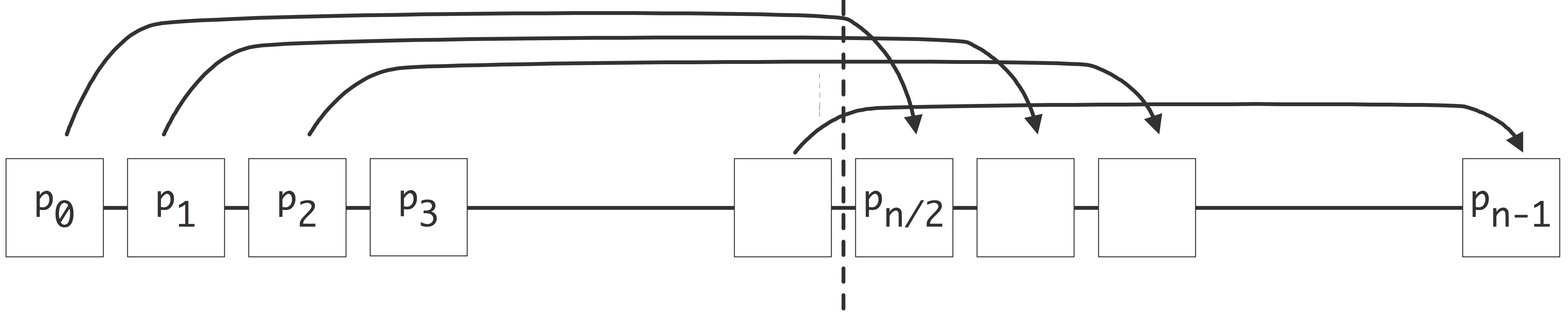

This sort of conflict is called congestion or contention  . Clearly, the more links a parallel computer has, the smaller the chance of congestion.

A precise way to describe the likelihood of congestion, is to look at the bisection width  . This is defined as the minimum number of links that have to be removed to partition the processor graph into two unconnected graphs. For instance, consider processors connected as a linear array, that is, processor $P_i$ is connected to $P_{i-1}$ and $P_{i+1}$. In this case the bisection width is 1.

The bisection width $w$ describes how many messages can, guaranteed, be under way simultaneously in a parallel computer. Proof: take $w$ sending and $w$ receiving processors. The $w$ paths thus defined are disjoint: if they were not, we could separate the processors into two groups by removing only $w-1$ links.

In practice, of course, more than $w$ messages can be under way simultaneously. For instance, in a linear array, which has $w=1$, $P/2$ messages can be sent and received simultaneously if all communication is between neighbors, and if a processor can only send or receive, but not both, at any one time. If processors can both send and receive simultaneously, $P$ messages can be under way in the network.

Bisection width also describes redundancy in a network: if one or more connections are malfunctioning, can a message still find its way from sender to receiver?

While bisection width is a measure expressing a number of wires, in practice we care about the capacity through those wires. The relevant concept here is bisection bandwidth : the bandwidth across the bisection width, which is the product of the bisection width, and the capacity (in bits per second) of the wires. Bisection bandwidth can be considered as a measure for the bandwidth that can be attained if an arbitrary half of the processors communicates with the other half. Bisection bandwidth is a more realistic measure than the aggregate bandwidth which is sometimes quoted and which is defined as the total data rate if every processor is sending: the number of processors times the bandwidth of a connection times the number of simultaneous sends a processor can perform. This can be quite a high number, and it is typically not representative of the communication rate that is achieved in actual applications.

2.7.2 Busses

crumb trail: > parallel > Topologies > Busses

The first interconnect design we consider is to have all processors on the same memory bus  . This design connects all processors directly to the same memory pool, so it offers a UMA or SMP model.

The main disadvantage of using a bus is the limited scalability, since only one processor at a time can do a memory access. To overcome this, we need to assume that processors are slower than memory, or that the processors have cache or other local memory to operate out of. In the latter case, maintaining cache coherence is easy with a bus by letting processors listen to all the memory traffic on the bus -- a process known as snooping  .

2.7.3 Linear arrays and rings

crumb trail: > parallel > Topologies > Linear arrays and rings

A simple way to hook up multiple processors is to connect them in a linear array processor $P_i$ is connected to $P_{i-1}$ and $P_{i+1}$. The first and last processor are possible exceptions: if they are connected to each other, we call the architecture a ring network  .

This solution requires each processor to have two network connections, so the design is fairly simple.

Exercise What is the bisection width of a linear array? Of a ring?
End of exercise

Exercise With the limited connections of a linear array, you may have to be clever about how to program parallel algorithms. For instance, consider a `broadcast' operation: processor $0$ has a data item that needs to be sent to every other processor.

We make the following simplifying assumptions:

• a processor can send any number of messages simultaneously,
• but a wire can can carry only one message at a time; however,
• communication between any two processors takes unit time, regardless of the number of processors in between them.

In a fully connected network or a star network you can simply write

  for $i=1\ldots N-1$: send the message to processor $i$

With the assumption that a processor can send multiple messages, this means that the operation is done in one step.

Now consider a linear array. Show that, even with this unlimited capacity for sending, the above algorithm runs into trouble because of congestion.

Find a better way to organize the send operations. Hint: pretend that your processors are connected as a binary tree. Assume that there are $N=2^n-1$ processors. Show that the broadcast can be done in $\log N$ stages, and that processors only need to be able to send a single message simultaneously.
End of exercise

This exercise is an example of embedding a `logical' communication pattern in a physical one.

2.7.4 2D and 3D arrays

crumb trail: > parallel > Topologies > 2D and 3D arrays

A popular design for parallel computers is to organize the processors in a two-dimensional or three-dimensional Cartesian mesh  . This means that every processor has a coordinate $(i,j)$ or $(i,j,k)$, and it is connected to its neighbors in all coordinate directions. The processor design is still fairly simple: the number of network connections (the degree of the connectivity graph) is twice the number of space dimensions (2 or 3) of the network.

It is a fairly natural idea to have 2D or 3D networks, since the world around us is three-dimensional, and computers are often used to model real-life phenomena. If we accept for now that the physical model requires nearest neighbor type communications (which we will see is the case in section  4.2.3  ), then a mesh computer is a natural candidate for running physics simulations.

Exercise What is the diameter of a 3D cube of $n\times n\times n$ processors? What is the bisection width? How does that change if you add wraparound torus connections?
End of exercise

Exercise Your parallel computer has its processors organized in a 2D grid. The chip manufacturer comes out with a new chip with same clock speed that is dual core instead of single core, and that will fit in the existing sockets. Critique the following argument: `the amount of work per second that can be done (that does not involve communication) doubles; since the network stays the same, the bisection bandwidth also stays the same, so I can reasonably expect my new machine to become twice as fast'.
End of exercise

Grid-based designs often have so-called wrap-around or torus connections, which connect the left and right sides of a 2D grid, as well as the top and bottom. This is illustrated in figure  2.16  .

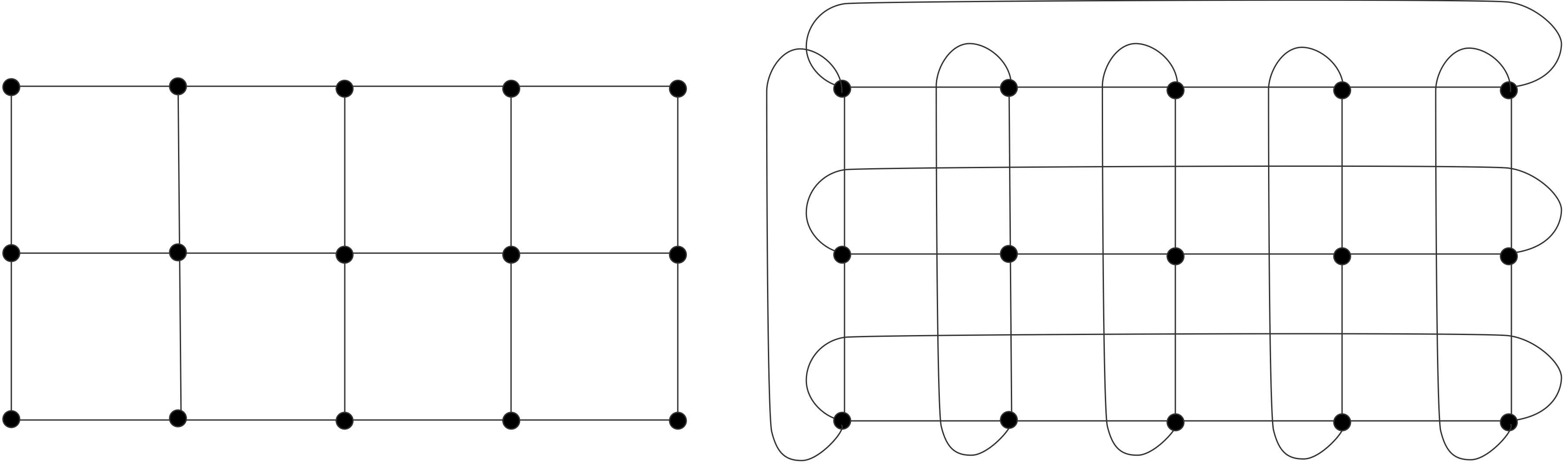
FIGURE 2.16: A 2D grid with torus connections.

Some computer designs claim to be a grid of high dimensionality, for instance 5D, but not all dimensions are equal here. For instance, a 3D grid where each node is a quad-socket quad-core can be considered as a 5D grid. However, the last two dimensions are fully connected.

2.7.5 Hypercubes

crumb trail: > parallel > Topologies > Hypercubes

Above we gave a hand-waving argument for the suitability of mesh-organized processors based on the prevalence of nearest neighbor communications. However, sometimes sends and receives between arbitrary processors occur. One example of this is the above-mentioned broadcast. For this reason, it is desirable to have a network with a smaller diameter than a mesh. On the other hand we want to avoid the complicated design of a fully connected network.

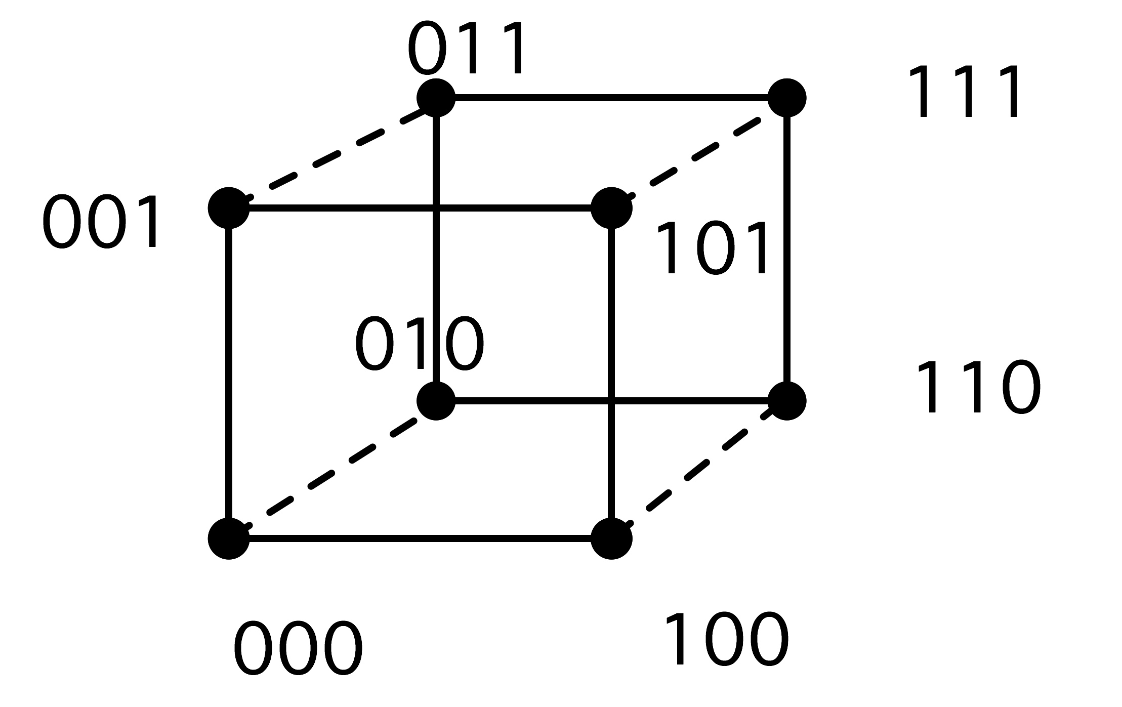
WRAPFIGURE 2.17: Numbering of the nodes of a hypercube.

A good intermediate solution is the hypercube design. An $n$-dimensional hypercube computer has $2^n$ processors, with each processor connected to one other in each dimension; see figure  2.18  .

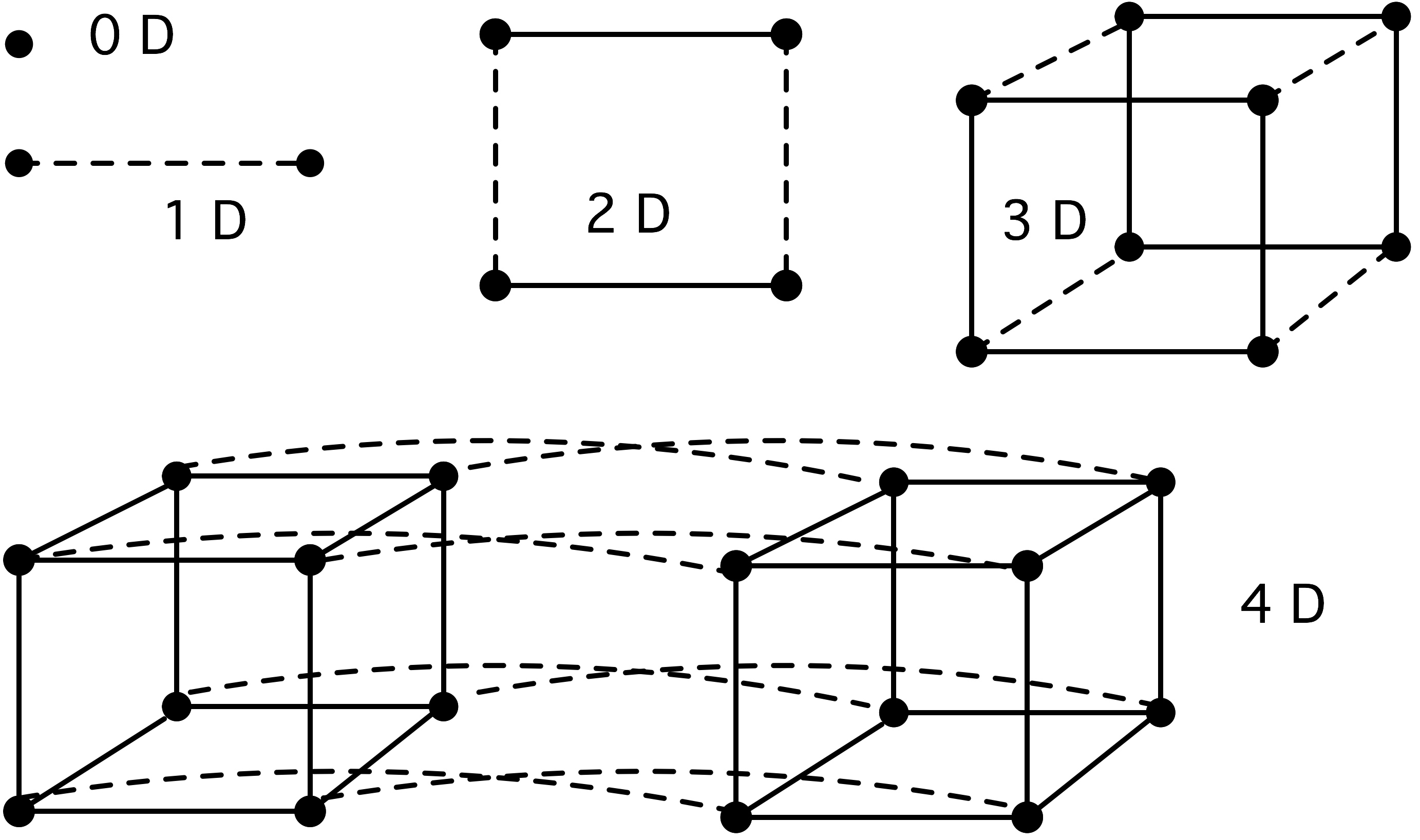
QUOTE 2.18: Hypercubes.

An easy way to describe this is to give each processor an address consisting of $d$ bits: we give each node of a hypercube a number that is the bit pattern describing its location in the cube; see figure  2.18  .

With this numbering scheme, a processor is then connected to all others that have an address that differs by exactly one bit. This means that, unlike in a grid, a processor's neighbors do not have numbers that differ by 1 or $\sqrt P$, but by $1,2,4,8,\ldots$.

The big advantages of a hypercube design are the small diameter and large capacity for traffic through the network.

Exercise What is the diameter of a hypercube? What is the bisection width?
End of exercise

One disadvantage is the fact that the processor design is dependent on the total machine size. In practice, processors will be designed with a maximum number of possible connections, and someone buying a smaller machine then will be paying for unused capacity. Another disadvantage is the fact that extending a given machine can only be done by doubling it: other sizes than $2^p$ are not possible.

Exercise Consider the parallel summing example of section  2.1  , and give the execution time of a parallel implementation on a hypercube. Show that the theoretical speedup from the example is attained (up to a factor) for the implementation on a hypercube.
End of exercise

2.7.5.1 Embedding grids in a hypercube

crumb trail: > parallel > Topologies > Hypercubes > Embedding grids in a hypercube

\def\graycodepicture{

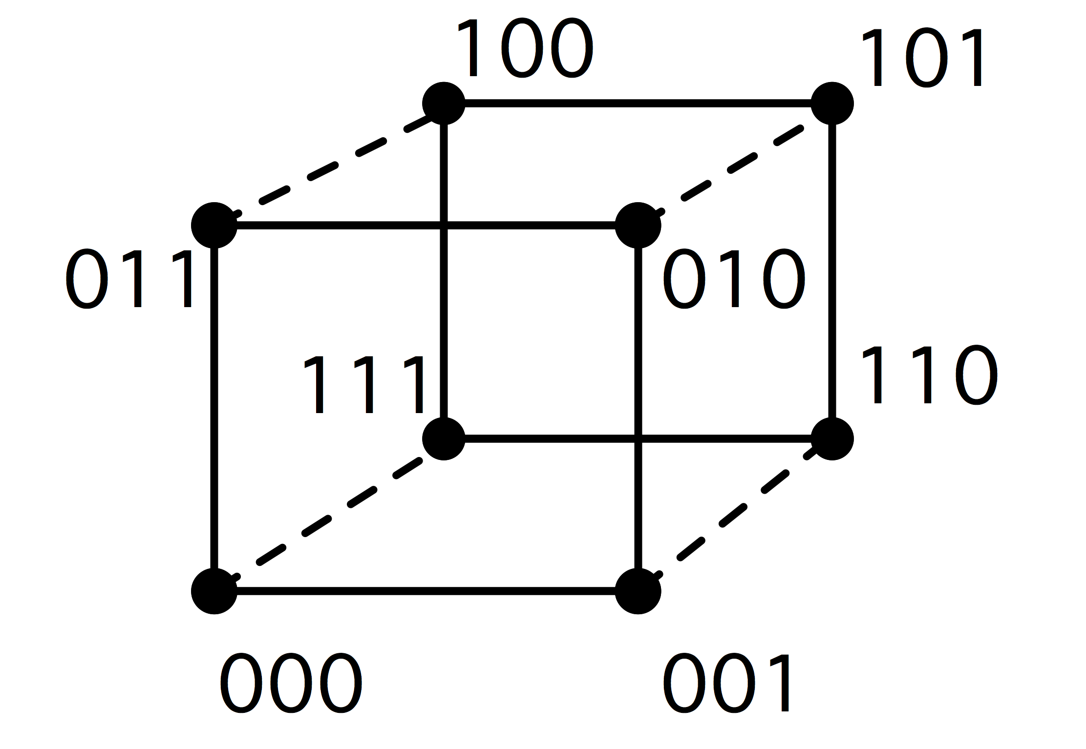
WRAPFIGURE 2.19: Gray code numbering of the nodes of a hypercube.

}

Above we made the argument that mesh-connected processors are a logical choice for many applications that model physical phenomena. Hypercubes do not look like a mesh, but they have enough connections that they can simply pretend to be a mesh by ignoring certain connections.

\newpage \graycodepicture

Let's say that we want the structure of a 1D array: we want processors with a numbering so that processor $i$ can directly send data to $i-1$ and $i+1$. We can not use the obvious numbering of nodes as in figure  2.18  . For instance, node 1 is directly connected to node 0, but has a distance of 2 to node 2. The right neighbor of node 3 in a ring, node 4, even has the maximum distance of 3 in this hypercube. Clearly we need to renumber the nodes in some way.

What we will show is that it's possible to walk through a hypercube, touching every corner exactly once, which is equivalent to embedding a 1D mesh in the hypercube.

\hbox{\fbox{1D Gray code}: $\vcenter{$ \begin{array}{rll}
hphantom{1D code and reflection:}&0&1

\end{array} $} $}

\hbox{\fbox{2D Gray code}: $\vcenter{$ \begin{array}{rccccc}
hbox{1D code and reflection:}&0&1&
vdots&1&0

\hbox{append 0 and 1 bit:}&0&0&\vdots&1&1 \end{array} $} $}

\hbox{\fbox{3D Gray code}: $\vcenter{$ \begin{array}{rccccccccc}
hbox{2D code and reflection:}&0&1&1&0&
vdots&0&1&1&0

&0&0&1&1&
vdots&1&1&0&0

\hbox{append 0 and 1 bit:}&0&0&0&0&\vdots&1&1&1&1 \end{array} $} $}

FIGURE 2.20: Gray codes.

The basic concept here is a (binary reflected) \indexterm{Gray code}  [Gray:graycodepatent]  . This is a way of ordering the binary numbers $0\ldots2^d-\nobreak1$ as $g_0,\ldots g_{2^d-1}$ so that $g_i$ and $g_{i+1}$ differ in only one bit. Clearly, the ordinary binary numbers do not satisfy this: the binary representations for 1 and 2 already differ in two bits. Why do Gray codes help us? Well, since $g_i$ and $g_{i+1}$ differ only in one bit, it means they are the numbers of nodes in the hypercube that are directly connected.

Figure  2.20 illustrates how to construct a Gray code. The procedure is recursive, and can be described informally as `divide the cube into two subcubes, number the one subcube, cross over to the other subcube, and number its nodes in the reverse order of the first one'. The result for a 2D cube is in figure  2.19  .

Since a Gray code offers us a way to embed a one-dimensional `mesh' into a hypercube, we can now work our way up.

Exercise Show how a square mesh of $2^{2d}$ nodes can be embedded in a hypercube by appending the bit patterns of the embeddings of two $2^d$ node cubes. How would you accommodate a mesh of $2^{d_1+d_2}$ nodes? A three-dimensional mesh of $2^{d_1+d_2+d_3}$ nodes?
End of exercise

2.7.6 Switched networks

crumb trail: > parallel > Topologies > Switched networks

\def\crossbarfig{

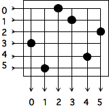
QUOTE 2.21: A simple cross bar connecting 6 inputs to 6 outputs.

}

Above, we briefly discussed fully connected processors. They are impractical if the connection is made by making a large number of wires between all the processors. There is another possibility, however, by connecting all the processors to a switch or switching network. Some popular network designs are the crossbar  , the butterfly exchange  , and the fat tree  .

Switching networks are made out of switching elements, each of which have a small number (up to about a dozen) of inbound and outbound links. By hooking all processors up to some switching element, and having multiple stages of switching, it then becomes possible to connect any two processors by a path through the network.

2.7.6.1 Cross bar

crumb trail: > parallel > Topologies > Switched networks > Cross bar

\crossbarfig

The simplest switching network is a cross bar, an arrangement of $n$ horizontal and vertical lines, with a switch element on each intersection that determines whether the lines are connected; see figure  2.21  . If we designate the horizontal lines as inputs the vertical as outputs, this is clearly a way of having $n$ inputs be mapped to $n$ outputs. Every combination of inputs and outputs (sometimes called a `permutation') is allowed.

One advantage of this type of network is that no connection blocks another. The main disadvantage is that the number of switching elements is $n^2$, a fast growing function of the number of processors $n$.

2.7.6.2 Butterfly exchange

crumb trail: > parallel > Topologies > Switched networks > Butterfly exchange

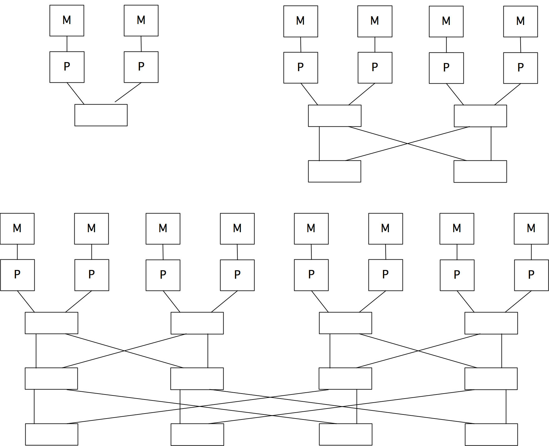\caption{Butterfly exchange networks for 2,4,8 processors, each with a local memory.}

Butterfly exchange elements, and they have multiple stages: as the number of processors grows, the number of stages grows with it. Figure  2.7.6.2 shows shows butterfly networks to connect 2,4, and 8 processors, each with a local memory. (Alternatively, you could put all processors at one side of the network, and all memories at the other.)

As you can see in figure  2.22  , butterfly exchanges allow several processors to access memory simultaneously. Also, their access times are identical, so exchange networks are a way of implementing a UMA architecture; see section  2.4.1  . One computer that was based on a Butterfly exchange network was the BBN Butterfly ( http://en.wikipedia.org/wiki/BBN_Butterfly  ). In section  2.7.7.1 we will see how these ideas are realized in a practical cluster.

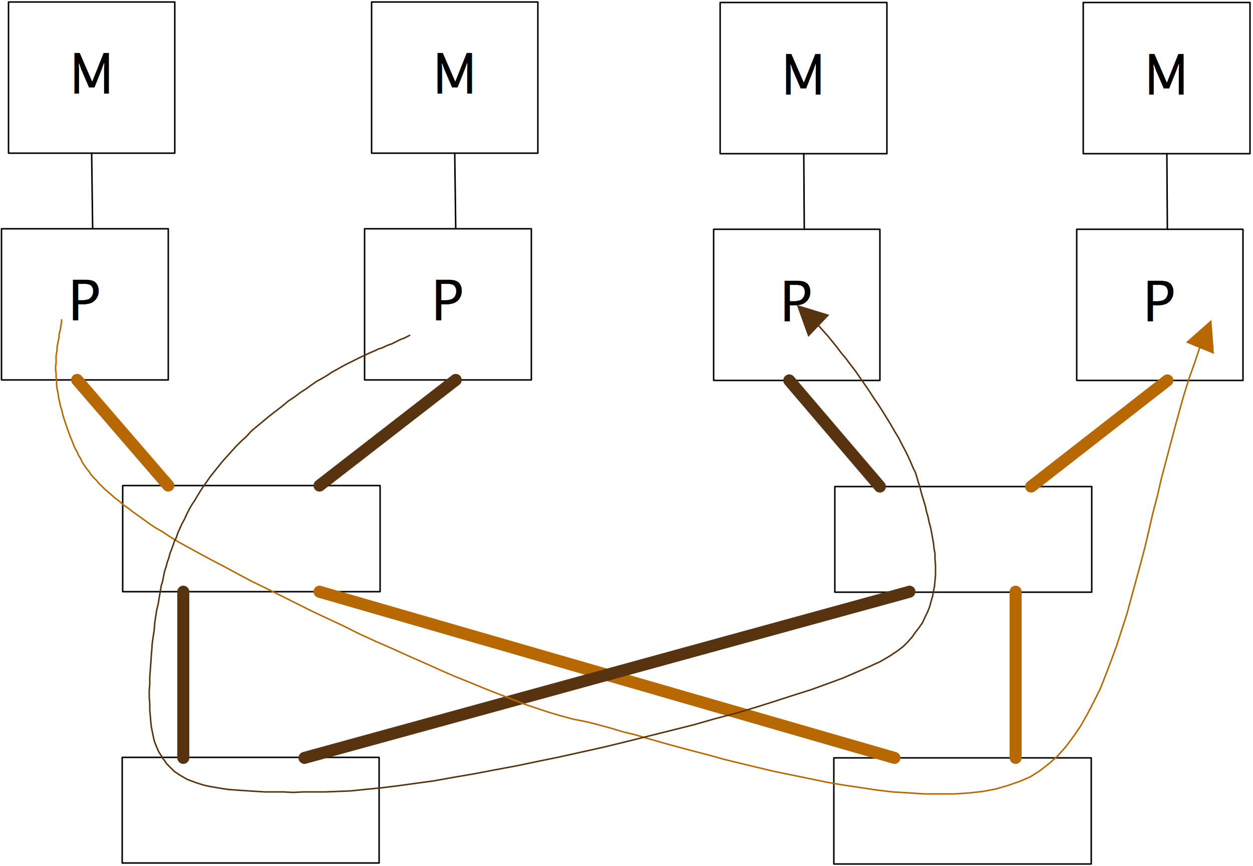
QUOTE 2.22: Two independent routes through a butterfly exchange network.

Exercise For both the simple cross bar and the butterfly exchange, the network needs to be expanded as the number of processors grows. Give the number of wires (of some unit length) and the number of switching elements that is needed in both cases to connect $n$ processors and memories. What is the time that a data packet needs to go from memory to processor, expressed in the unit time that it takes to traverse a unit length of wire and the time to traverse a switching element?
End of exercise

Packet routing network is done based on considering the bits in the destination address. On the $i$-th level the $i$-th digit is considered;

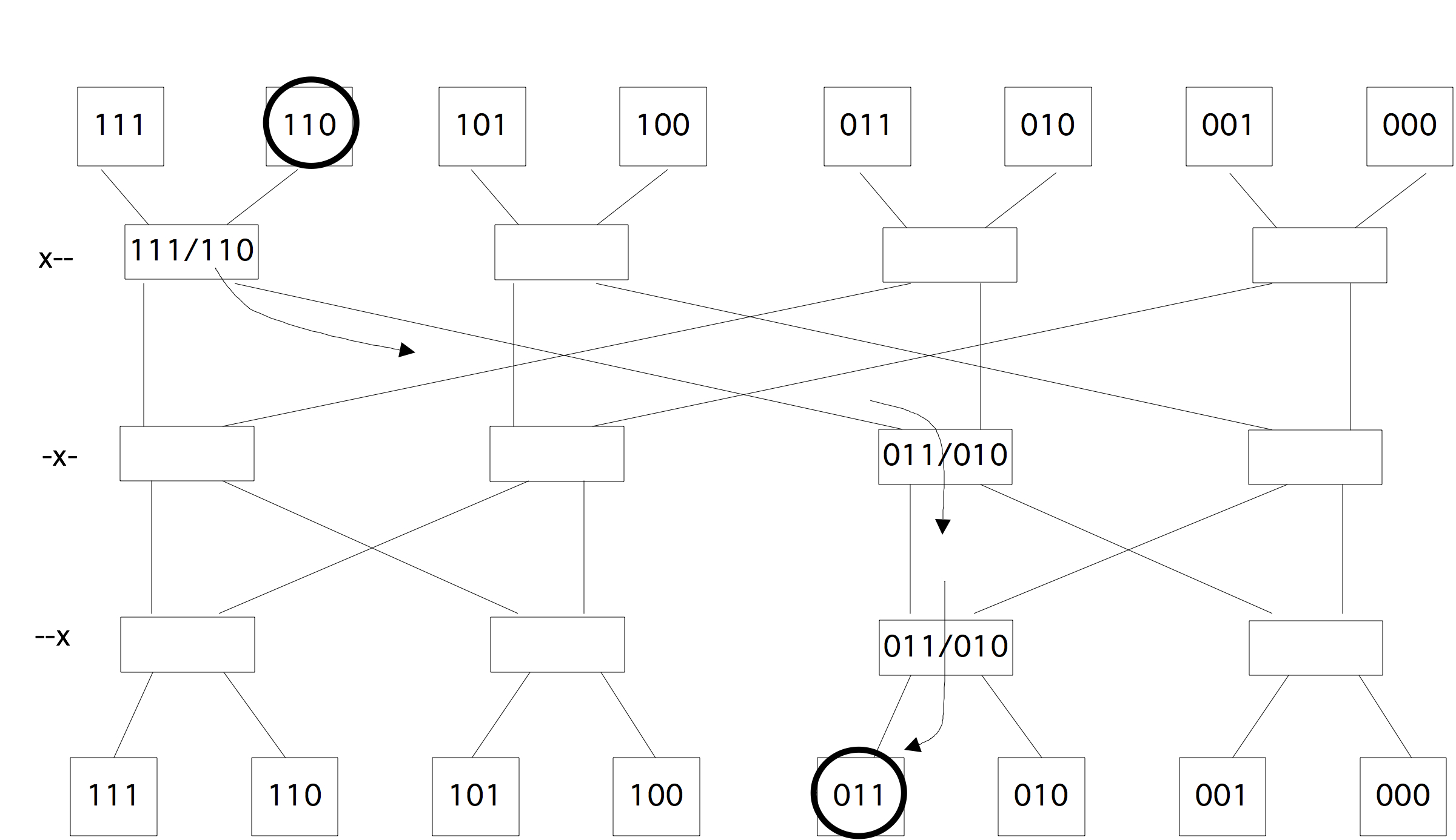
FIGURE 2.23: Routing through a three-stage butterfly exchange network.

if this is $1$, the left exit of the switch is taken, if $0$, the right exit. This is illustrated in figure  2.23  . If we attach the memories to the processors, as in figure  2.22  , we need only two bits (to the last switch) but a further three bits to describe the reverse route.

2.7.6.3 Fat-trees

crumb trail: > parallel > Topologies > Switched networks > Fat-trees

If we were to connect switching nodes like a tree, there would be a big problem with congestion close to the root since there are only two wires attached to the root note. Say we have a $k$-level tree, so there are $2^k$ leaf nodes. If all leaf nodes in the left subtree try to communicate with nodes in the right subtree, we have $2^{k-1}$ messages going through just one wire into the root, and similarly out through one wire. A fat-tree is a tree network where each level has the same total bandwidth, so that this congestion problem does not occur: the root will actually have $2^{k-1}$ incoming and outgoing wires attached  [Greenberg89randomizedrouting]  . Figure  2.7.6.3 shows this structure on the left;

\hbox{% 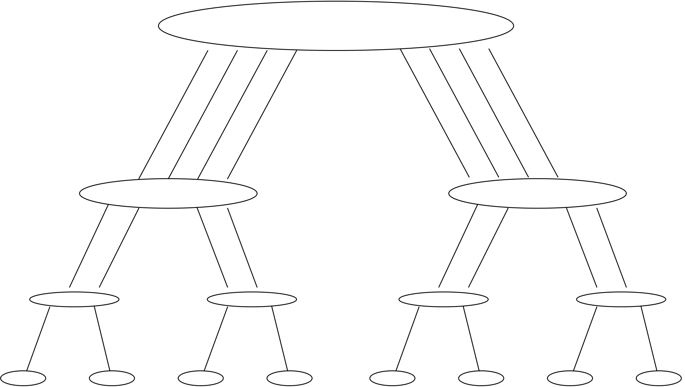\kern20pt \includegraphics{stampede_leaf} }

\caption{A fat tree with a three-level interconnect (left); the leaf switches in a cabinet of the Stampede cluster (right).}

on the right is shown a cabinet of the {Stampede cluster}, with a leaf switch for top and bottom half of the cabinet.

The first successful computer architecture based on a fat-tree was the Connection Machines CM5.

In fat-trees, as in other switching networks, each message carries its own routing information. Since in a fat-tree the choices are limited to going up a level, or switching to the other subtree at the current level, a message needs to carry only as many bits routing information as there are levels, which is $\log_2n$ for $n$ processors.

Exercise Show that the bisection width of a fat tree is $P/2$ where $P$ is the number of processor leaf nodes. Hint: show that there is only one way of splitting a fat tree-connected set of processors into two connected subsets.
End of exercise

The theoretical exposition of fat-trees in  [Leiserson:fattree] shows that fat-trees are optimal in some sense: it can deliver messages as fast (up to logarithmic factors) as any other network that takes the same amount of space to build. The underlying assumption of this statement is that switches closer to the root have to connect more wires, therefore take more components, and correspondingly are larger. This argument, while theoretically interesting, is of no practical significance, as the physical size of the network hardly plays a role in the biggest currently available computers that use fat-tree interconnect. For instance, in the TACC Frontera cluster at The University of Texas at Austin, there are only 6 core switch es (that is, cabinents housing the top levels of the fat tree), connecting 91 processor cabinets.

A fat tree, as sketched above, would be costly to build, since for every next level a new, bigger, switch would have to be designed. In practice, therefore, a network with the characteristics of a fat-tree is constructed from simple switching elements; see figure  2.24  .

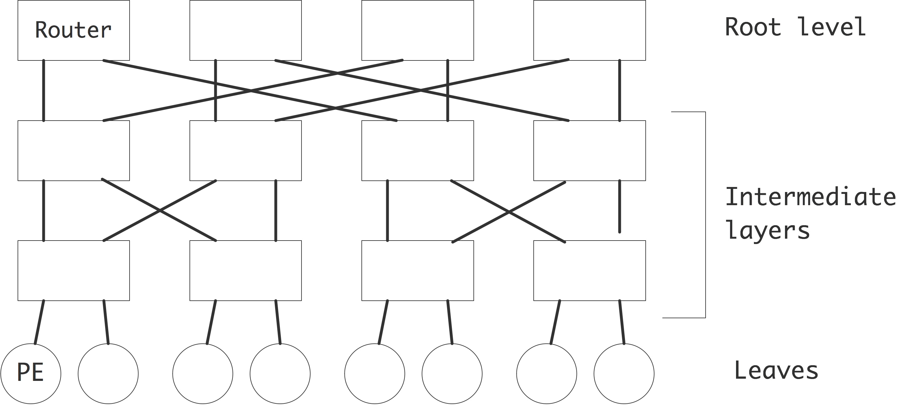
QUOTE 2.24: A fat-tree built from simple switching elements.

This network is equivalent in its bandwidth and routing possibilities to a fat-tree. Routing algorithms will be slightly more complicated: in a fat-tree, a data packet can go up in only one way, but here a packet has to know to which of the two higher switches to route.

This type of switching network is one case of a \indexterm{Clos network}  [Clos1953]  .

2.7.6.4 Over-subscription and contention

crumb trail: > parallel > Topologies > Switched networks > Over-subscription and contention

In practice, fat-tree networks do not use 2-in-2-out elements, but switches that are more on the order of 20-in-20-out. This makes it possible for the number of levels in a network to be limited to 3 or 4. (The top level switches are known as spine card s.)

An extra complication to the analysis of networks in this case is the possibility of oversubscription  . The ports in a network card are configurable as either in or out, and only the total is fixed. Thus, a 40-port switch can be configured as 20-in and 20-out, or 21-in and 19-out, et cetera. Of course, if all 21 nodes connected to the switch send at the same time, the 19 out ports will limit the bandwdidth.

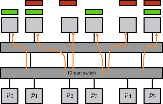
FIGURE 2.25: Port contention in an over-subscribed switch.

There is a further problem. Let us considering building a small cluster with switches configured to have $p$ in-ports and $w$ out-ports, meaning we have $p+w$-port switches. Figure  2.25 depicts two of such switching, connecting a total of $2p$ nodes. If a node sends data through the switch, its choice of the $w$ available wires is determined by the target node. This is known as output routing  .

Clearly we can only expect $w$ nodes to be able to send with message collisions, since that is the number of available wires between the switches. However, for many choices of $w$ targets there will be contention for the wires regardless. This is an example of the birthday paradox  .

Exercise Consider the above architecture with $p$ nodes sending through $w$ wires between the switching. Code a simulation where $w'\leq w$ out of $p$ nodes send a message to a randomly selected target node. What is the probability of collision as a function of $w',w,p$? Find a way to tabulate or plot data.

For bonus points, give a statistical analysis of the simple case $w'=2$.

End of exercise

2.7.7 Cluster networks

crumb trail: > parallel > Topologies > Cluster networks

The above discussion was somewhat abstract, but in real-life clusters you can actually see the network designs reflected. For instance, fat tree cluster networks

\hbox{% }

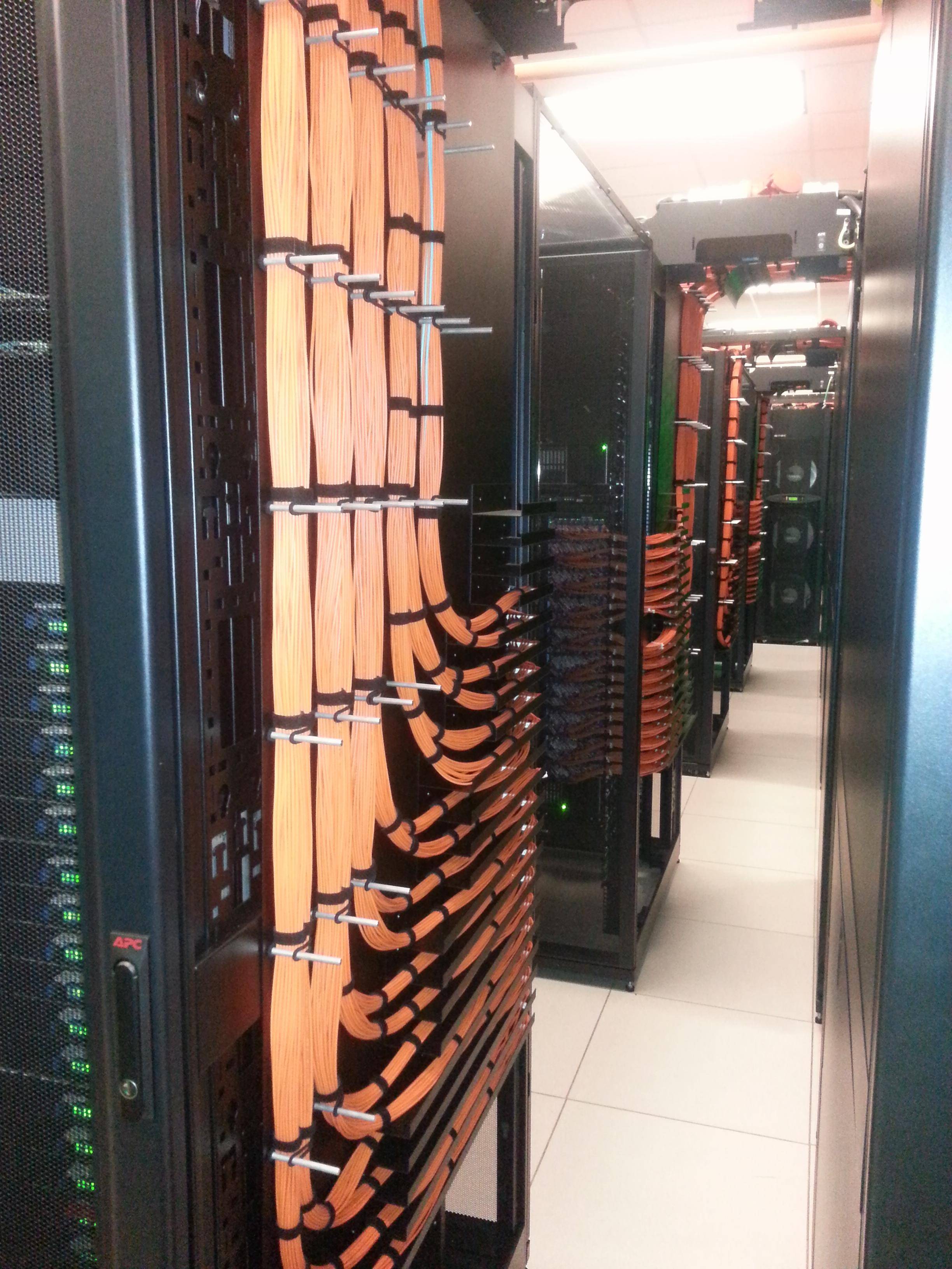FIGURE 2.26: Networks switches for the TACC Ranger and Stampede clusters.

will have a central cabinet corresponding to the top level in the tree. Figure  2.26 shows the switches of the TACC Ranger and Stampede clusters. In the second picture it can be seen that there are actually multiple redundant fat-tree networks.

On the other hand, clusters such as the IBM BlueGene  , which is based on a torus-based cluster  , will look like a collection of identical cabinets, since each contains

FIGURE 2.27: A BlueGene computer.

an identical part of the network; see figure  2.27  .

2.7.7.1 Case study: Stampede

crumb trail: > parallel > Topologies > Cluster networks > Case study: Stampede

As an example of networking in practice, let's consider the Stampede Advanced Computing Center. This can be described as a multi-root multi-stage fat-tree.

• Each rack consists of 2 chassis, with 20 nodes each.
• Each chassis has a leaf switch that is an internal crossbar that gives perfect connectivity between the nodes in a chassis;
• The leaf switch has 36 ports, with 20 connected to the nodes and 16 outbound. This oversubscription implies that at most 16 nodes can have perfect bandwidth when communicating outside the chassis.
• There are 8 central switches that function as 8 independent fat-tree root. Each chassis is connected by two connections to a `leaf card' in each of the central switches, taking up precisely the 16 outbound ports.
• Each central switch has 18 spine cards with 36 ports each, with each port connecting to a different leaf card.
• Each central switch has 36 leaf cards with 18 ports to the leaf switches and 18 ports to the spine cards. This means we can support 648 chassis, of which 640 are actually used.

One of the optimizations in the network is that two connections to the same leaf card communicate without the latency of the higher tree levels. This means that 16 nodes in one chassis and 16 nodes in another can have perfect connectivity.

However, with static routing  , such as used in Infiniband  , there is a fixed port associated with each destination. (This mapping of destination to port is in the routing tables in each switch.) Thus, for some subsets of 16 nodes out 20 possible destination there will be perfect bandwidth, but other subsets will see the traffic for two destinations go through the same port.

2.7.7.2 Case study: Cray Dragonfly networks

crumb trail: > parallel > Topologies > Cluster networks > Case study: Cray Dragonfly networks

The \indextermbusdef{Cray}{Dragonfly} network is an interesting practical compromise. Above we argued that a fully connected network would be too expensive to scale up. However, it is possible to have a fully connected set of processors, if the number stays limited. The Dragonfly design uses small fully connected groups, and then makes a fully connected graph of these groups.

This introduces an obvious asymmetry, since processors inside a group have a larger bandwidth then between groups. However, thanks to dynamic routing messages can take a non-minimal path, being routed through other groups. This can alleviate the contention problem.

2.7.8 Bandwidth and latency

crumb trail: > parallel > Topologies > Bandwidth and latency

The statement above that sending a message can be considered a unit time operation, is of course unrealistic. A large message will take longer to transmit than a short one. There are two concepts to arrive at a more realistic description of the transmission process; we have already seen this in section  1.3.2 in the context of transferring data between cache levels of a processor.

• [latency] Setting up a communication between two processors takes an amount of time that is independent of the message size. The time that this takes is known as the latency of a message. There are various causes for this delay.
  • The two processors engage in `hand-shaking', to make sure that the recipient is ready, and that appropriate buffer space is available for receiving the message.
  • The message needs to be encoded for transmission by the sender, and decoded by the receiver.
  • The actual transmission may take time: parallel computers are often big enough that, even at lightspeed, the first byte of a message can take hundreds of cycles to traverse the distance between two processors.
• [bandwidth] After a transmission between two processors has been initiated, the main number of interest is the number of bytes per second that can go through the channel. This is known as the bandwidth  . The bandwidth can usually be determined by the channel rate  , the rate at which a physical link can deliver bits, and the channel width  , the number of physical wires in a link. The channel width is typically a multiple of 16, usually 64 or 128. This is also expressed by saying that a channel can send one or two 8-byte words simultaneously.

Bandwidth and latency are formalized in the expression \begin{equation} T(n)=\alpha+\beta n \end{equation} for the transmission time of an $n$-byte message. Here, $\alpha$ is the latency and $\beta$ is the time per byte, that is, the inverse of bandwidth. Sometimes we consider data transfers that involve communication, for instance in the case of a \indexterm{collective operation}; see section  6.1  . We then extend the transmission time formula to \begin{equation} T(n)=\alpha+\beta n+\gamma n \end{equation} where $\gamma$ is the time per operation, that is, the inverse of the computation rate  .

It would also be possible to refine this formulas as \begin{equation} T(n,p) = \alpha+\beta n+\delta p \end{equation} where $p$ is the number of network `hops' that is traversed. However, on most networks the value of $\delta$ is far lower than of $\alpha$, so we will ignore it here. Also, in fat-tree networks (section  2.7.6.3  ) the number of hops is of the order of $\log P$, where $P$ is the total number of processors, so it can never be very large anyway.

2.7.9 Locality in parallel computing

crumb trail: > parallel > Topologies > Locality in parallel computing

In section  1.6.2 you found a discussion of locality concepts in single-processor computing. The concept of locality in parallel computing comprises all this and a few levels more.

Between cores; private cache
Cores on modern processors have private coherent caches. This means that it looks like you don't have to worry about locality, since data is accessible no matter what cache it is in. However, maintaining coherence costs bandwidth, so it is best to keep access localized.

Between cores; shared cache
The cache that is shared between cores is one place where you don't have to worry about locality: this is memory that is truly symmetric between the processing cores.

Between sockets
The sockets on a node (or motherboard) appear to the programmer to have shared memory, but this is really NUMA access (section  2.4.2  ) since the memory is associated with specific sockets.

Through the network structure
Some networks have clear locality effects. You saw a simple example in section  2.7.1  , and in general it is clear that any grid-type network will favor communication between `nearby' processors. Networks based on fat-trees seem free of such contention issues, but the levels induce a different form of locality. One level higher than the locality on a node, small groups of nodes are often connected by a leaf switch  , which prevents data from going to the central switch.

2.8 Multi-threaded architectures

crumb trail: > parallel > Multi-threaded architectures

The architecture of modern CPUs is largely dictated by the fact that getting data from memory is much slower than processing it. Hence, a hierarchy of ever faster and smaller memories tries to keep data as close to the processing unit as possible, mitigating the long latency and small bandwidth of main memory. The ILP in the processing unit also helps to hide the latency and more fully utilize the available bandwidth.

However, finding ILP is a job for the compiler and there is a limit to what it can practically find. On the other hand, scientific codes are often very data parallel in a sense that is obvious to the programmer, though not necessarily to the compiler. Would it be possible for the programmer to specify this parallelism explicitly and for the processor to use it?

In section  2.3.1 you saw that SIMD architectures can be programmed in an explicitly data parallel way. What if we have a great deal of data parallelism but not that many processing units? In that case, we could turn the parallel instruction streams into threads (see section  2.6.1  ) and have multiple threads be executed on each processing unit. Whenever a thread would stall because of an outstanding memory request, the processor could switch to another thread for which all the necessary inputs are available. This is called multi-threading  . While it sounds like a way of preventing the processor from waiting for memory, it can also be viewed as a way of keeping memory maximally occupied.

Exercise If you consider the long latency and limited bandwidth of memory as two separate problems, does multi-threading address them both?
End of exercise

The problem here is that most CPUs are not good at switching quickly between threads. A  context switch (switching between one thread and another) takes a large number of cycles, comparable to a wait for data from main memory. In a so-called MTA a context-switch is very efficient, sometimes as little as a single cycle, which makes it possible for one processor to work on many threads simultaneously.

The multi-threaded concept was explored in the \indextermbus{Tera Computer}{MTA} machine, which evolved into the current Cray XMT

(Note: {Tera Computer renamed itself Cray Inc. after acquiring Cray Research from SGI  .}  )

.

The other example of an MTA is the GPU  , where the processors work as SIMD units, while being themselves multi-threaded; see section  2.9.3  .

2.9 Co-processors, including GPUs

crumb trail: > parallel > Co-processors, including GPUs

Current CPUs are built to be moderately efficient at just about any conceivable computation. This implies that by restricting the functionality of a processor it may be possible to raise its efficiency, or lower its power consumption at similar efficiency. Thus, the idea of incorporating a co-processor attached to the host process has been explored many times. For instance, Intel's 8086 chip, which powered the first generation of IBM PCs, could have a numerical co-processor, the 80287, added to it. This processor was very efficient at transcendental functions and it also incorporated SIMD technology. Using separate functionality for graphics has also been popular, leading to the SSE instructions for the x86 processor, and separate GPU units to be attached to the PCI-X bus.

Further examples are the use of co-processors for DSP instructions, as well as FPGA boards which can be reconfigured to accommodate specific needs. Early array processors such as the ICL DAP were also co-processors.

In this section we look briefly at some modern incarnations of this idea, in particular GPUs  .

2.9.1 A little history

crumb trail: > parallel > Co-processors, including GPUs > A little history

Co-processors can be programmed in two different ways: sometimes it is seamlessly integrated, and certain instructions are automatically executed there, rather than on the `host' processor. On the other hand, it is also possible that co-processor functions need to be explicitly invoked, and it may even be possible to overlap co-processor functions with host functions. The latter case may sound attractive from an efficiency point of view, but it raises a serious problem of programmability. The programmer now needs to identify explicitly two streams of work: one for the host processor and one for the co-processor.

Some notable parallel machines with co-processors are:

• The Intel Paragon (1993) had two processors per node, one for communication and the other for computation. These were in fact identical, the Intel i860 Intel i860 processor. In a later revision, it became possible to pass data and function pointers to the communication processors.
• The IBM Roadrunner at Los Alamos was the first machine to reach a PetaFlop. (The Grape computer had reached this point earlier, but that was a special purpose machine for molecular dynamics calculations.) It achieved this speed through the use of Cell co-processors. Incidentally, the Cell processor is in essence the engine of the Sony Playstation3, showing again the commoditization of supercomputers (section  2.3.3  ).
• The Chinese Tianhe-1A topped the Top 500 list in 2010, reaching about 2.5 PetaFlops through the use of NVidia GPUs  .
• The Tianhe-2 and the TACC Stampede cluster use Intel Xeon Phi co-processors.

The Roadrunner and Tianhe-1A are examples of co-processors that are very powerful, and that need to be explicitly programmed independently of the host CPU. For instance, code running on the GPUs of the Tianhe-1A is programmed in CUDA and compiled separately.

In both cases the programmability problem is further exacerbated by the fact that the co-processor can not directly talk to the network. To send data from one co-processor to another it has to be passed to a host processor, from there through the network to the other host processor, and only then moved to the target co-processor.

2.9.2 Bottlenecks

crumb trail: > parallel > Co-processors, including GPUs > Bottlenecks

Co-processors often have their own memory, and the Intel Xeon Phi can run programs independently, but more often there is the question of how to access the memory of the host processor. A popular solution is to connect the co-processor through a PCI bus  . Accessing host memory this way is slower than the direct connection that the host processor has. For instance, the Intel Xeon Phi has a bandwidth 5.5GT per second (we will get to that `GT' in a second), while its connection to host memory is 5.0GT/s, but only 16-bit wide.

GT measure
We are used to seeing bandwidth measured in gigabits per second. For a PCI bus one often see the GT measure. This stands for giga-transfer, and it measures how fast the bus can change state between zero and one. Normally, every state transition would correspond to a bit, except that the bus has to provide its own clock information, and if you would send a stream of identical bits the clock would get confused. Therefore, every 8 bits are encoded in 10 bits, to prevent such streams. However, this means that the effective bandwidth is lower than the theoretical number, by a factor of $4/5$ in this case.

And since manufacturers like to give a positive spin on things, they report the higher number.

2.9.3 GPU computing

crumb trail: > parallel > Co-processors, including GPUs > GPU computing

A GPU (or sometimes GPGPU  ) is a special purpose processor, designed for fast graphics processing. However, since the operations done for graphics are a form of arithmetic, GPUs have gradually evolved a design that is also useful for non-graphics computing. The general design of a GPU is motivated by the `graphics pipeline': identical operations are performed on many data elements in a form of data parallelism (section  2.5.1  ), and a number of such blocks of data parallelism can be active at the same time.

WRAPFIGURE 2.28: Memory structure of a GPU.

The basic limitations that hold for a CPU hold for a GPU : accesses to memory incur a long latency. The solution to this problem in a CPU is to introduce levels of cache; in the case of a GPU a different approach is taken (see also section  2.8  ). GPUs are concerned with throughput computing  , delivering large amounts of data with high average rates, rather than any single result as quickly as possible. This is made possible by supporting many threads (section  2.6.1  ) and having very fast switching between them. While one thread is waiting for data from memory, another thread that already has its data can proceed with its computations.

2.9.3.1 SIMD-type programming with kernels

crumb trail: > parallel > Co-processors, including GPUs > GPU computing > SIMD-type programming with kernels

Present day GPUs

(Note: {The most popular GPUs today are made by NVidia, and are programmed in CUDA  , an extension of the C language.}  )

have an architecture that combines SIMD and SPMD parallelism. Threads are not completely independent, but are ordered in thread blocks  , where all threads in the block execute the same instruction, making the execution SIMD  . It is also possible to schedule the same instruction stream (a `kernel' in Cuda terminology) on more than one thread block. In this case, thread blocks can be out of sync, much like processes in an SPMD context. However, since we are dealing with threads here, rather than processes, the term SIMT is used.

This software design is apparent in the hardware; for instance, an NVidia GPU has 16--30 SMs  , and a SMs consists of 8 SPs  , which correspond to processor cores; see figure  2.29  . The SPs act in true SIMD fashion. The number of cores in a GPU is typically larger than in traditional multi-core processors, but the cores are more limited. Hence, the term manycore is used here.

QUOTE 2.29: Diagram of a GPU.

The SIMD  , or data parallel  , nature of GPUs becomes apparent in the way CUDA starts processes. A  kernel  , that is, a function that will be executed on the GPU  , is started on $mn$ cores by:

KernelProc<< m,n >>(args)

The collection of $mn$ cores executing the kernel is known as a grid $m$  thread blocks of $n$ threads each. A thread block can have up to 512 threads.

Recall that threads share an address space (see section  2.6.1  ), so they need a way to identify what part of the data each thread will operate on. For this, the blocks in a thread are numbered with $x,y$ coordinates, and the threads in a block are numbered with $x,y,z$ coordinates. Each thread knows its coordinates in the block, and its block's coordinates in the grid.

We illustrate this with a vector addition example:

// Each thread performs one addition
__global__ void vecAdd(float* A, float* B, float* C)
{
  int i = threadIdx.x + blockDim.x * blockIdx.x;
  C[i] = A[i] + B[i];
}
int main()
{
  // Run grid of N/256 blocks of 256 threads each
  vecAdd<<< N/256, 256>>>(d_A, d_B, d_C);
}

This shows the SIMD nature of GPUs : every thread executes the same scalar program, just on different data.

FIGURE 2.30: Thread indexing in CUDA.

Threads in a thread block are truly data parallel: if there is a conditional that makes some threads take the true branch and others the false branch, then one branch will be executed first, with all threads in the other branch stopped. Subsequently, and not simultaneously then execute their code. This may induce a severe performance penalty.

GPUs rely on a large amount of data parallelism and the ability to do a fast context switch  . This means that they will thrive in graphics and scientific applications, where there is lots of data parallelism. However they are unlikely to do well on `business applications' and operating systems, where the parallelism is of the ILP type, which is usually limited.

2.9.3.2 GPUs versus CPUs

crumb trail: > parallel > Co-processors, including GPUs > GPU computing > GPUs versus CPUs

These are some of the differences between GPUs and regular CPUs:

• First of all, as of this writing (late 2010), GPUs are attached processors, for instance over a PCI-X bus  , so any data they operate on has to be transferred from the CPU. Since the memory bandwidth of this transfer is low, at least 10 times lower than the memory bandwidth in the GPU  , sufficient work has to be done on the GPU to overcome this overhead.
• Since GPUs are graphics processors, they put an emphasis on single precision floating point arithmetic. To accommodate the scientific computing community, \indexterm{double precision} support is increasing, but double precision speed is typically half the single precision flop rate. This discrepancy is likely to be addressed in future generations.
• A CPU is optimized to handle a single stream of instructions that can be very heterogeneous in character; a  GPU is made explicitly for data parallelism, and will perform badly on traditional codes.
• A CPU is made to handle one thread  , or at best a small number of threads. A  GPU needs a large number of threads, far larger than the number of computational cores, to perform efficiently.

2.9.3.3 Expected benefit from GPUs

crumb trail: > parallel > Co-processors, including GPUs > GPU computing > Expected benefit from GPUs

GPUs have rapidly gained a reputation for achieving high performance, highly cost effectively. Stories abound of codes that were ported with minimal effort to CUDA, with a resulting speedup of sometimes $400$ times. Is the GPU really such a miracle machine? Were the original codes badly programmed? Why don't we use GPUs for everything if they are so great?

The truth has several aspects.

First of all, a GPU is not as general-purpose as a regular CPU: GPUs are very good at doing data parallel computing, and CUDA is good at expressing this fine-grained parallelism elegantly. In other words, GPUs are suitable for a certain type of computation, and will be a poor fit for many others.

Conversely, a regular CPU is not necessarily good at data parallelism. Unless the code is very carefully written, performance can degrade from optimal by approximately the following factors:

• Unless directives or explicit parallel constructs are used, compiled code will only use 1 out of the available cores, say 4.
• If instructions are not pipelined, the latency because of the floating point pipeline adds another factor of 4.
• If the core has independent add and multiply pipelines, another factor of 2 will be lost if they are not both used simultaneously.
• Failure to use SIMD registers can add more to the slowdown with respect to peak performance.

Writing the optimal CPU implementation of a computational kernel often requires writing in assembler, whereas straightforward CUDA code will achieve high performance with comparatively little effort, provided of course the computation has enough data parallelism.

2.9.4 Intel Xeon Phi

crumb trail: > parallel > Co-processors, including GPUs > Intel Xeon Phi

Intel Xeon Phi (also known by its architecture design as MIC  ) is a design expressly designed for numerical computing. The initial design, the Knights Corner

was a co-processor, though the second iteration, the Knights Landing

was self-hosted.

As a co-processor, the Xeon Phi has both differences and similarities with GPUs  .

• Both are connected through a PCI-X bus, which means that operations on the device have a considerable latency in starting up.
• The Xeon Phi has general purpose cores, so that it can run whole programs; GPUs has that only to a limited extent (see section  2.9.3.1  ).
• The Xeon Phi accepts ordinary C code.
• Both architectures require a large amount of SIMD-style parallelism, in the case of the Xeon Phi because of the 8-word wide AVX instructions.
• Both devices work, or can work, through offloading from a host program. In the case of the Xeon Phi this can happen with OpenMP constructs and MKL calls.

2.10 Load balancing

crumb trail: > parallel > Load balancing

In much of this chapter, we assumed that a problem could be perfectly divided over processors, that is, a processor would always be performing useful work, and only be idle because of latency in communication. In practice, however, a processor may be idle because it is waiting for a message, and the sending processor has not even reached the send instruction in its code. Such a situation, where one processor is working and another is idle, is described as load unbalance : there is no intrinsic reason for the one processor to be idle, and it could have been working if we had distributed the work load differently.

There is an asymmetry between processors having too much work and having not enough work: it is better to have one processor that finishes a task early, than having one that is overloaded so that all others wait for it.

Exercise Make this notion precise. Suppose a parallel task takes time 1 on all processors but one.

• Let $0<\alpha<1$ and let one processor take time $1+\alpha$. What is the speedup and efficiency as function of the number of processors? Consider this both in the Amdahl and Gustafsson sense (section  2.2.3  ).
• Answer the same questions if one processor takes time $1-\alpha$.

End of exercise

Load balancing is often expensive since it requires moving relatively large amounts of data. For instance, section  6.5 has an analysis showing that the data exchanges during a sparse matrix-vector product is of a lower order than what is stored on the processor. However, we will not go into the actual cost of moving: our main concerns here are to balance the workload, and to preserve any locality in the original load distribution.

2.10.1 Load balancing versus data distribution

crumb trail: > parallel > Load balancing > Load balancing versus data distribution

There is a duality between work and data: in many applications the distribution of data implies a distribution of work and the other way around. If an application updates a large array, each element of the array typically `lives' on a uniquely determined processor, and that processor takes care of all the updates to that element. This strategy is known as owner computes  .

Thus, there is a direct relation between data and work, and, correspondingly, data distribution and load balancing go hand in hand. For instance, in section  6.2 we will talk about how data distribution influences the efficiency, but this immediately translates to concerns about load distribution:

• Load needs to be evenly distributed. This can often be done by evenly distributing the data, but sometimes this relation is not linear.
• Tasks need to be placed to minimize the amount of traffic between them. In the matrix-vector multiplication case this means that a two-dimensional distribution is to be preferred over a one-dimensional one; the discussion about space-filling curves is similarly motivated.

As a simple example of how the data distribution influences the load balance, consider a linear array where each point undergoes the same computation, and each computation takes the same amount of time. If the length of the array, $N$, is perfectly divisible by the number of processors, $p$, the work is perfectly evenly distributed. If the data is not evenly divisible, we start by assigning $\lfloor N/p\rfloor$ points to each processor, and the remaining $N-p\lfloor N/p\rfloor$ points to the last processors.

Exercise In the worst case, how unbalanced does that make the processors' work? Compare this scheme to the option of assigning $\lceil N/p\rceil$ points to all processors except one, which gets fewer; see the exercise above.
End of exercise

It is better to spread the surplus $r=N-p\lfloor N/p\rfloor$ over $r$ processors than one. This could be done by giving one extra data point to the first or last $r$ processors. This can be achieved by assigning to process $p$ the range \begin{equation} \bigl[ p\times \lfloor (N+p-1)/p \rfloor, (p+1)\times \lfloor (N+p-1)/p \rfloor \bigr) \end{equation} While this scheme is decently balanced, computing for instance to what processor a given point belongs is tricky. The following scheme makes such computations easier: let $f(i)=\lfloor iN/p\rfloor$, then processor $i$ gets points $f(i)$ up to $f(i+1)$.

Exercise Show that $\lfloor N/p\rfloor \leq f(i+1)-f(i)\leq \lceil N/p\rceil$.
End of exercise

Under this scheme, the processor that owns index $i$ is $\lfloor (p(i+1)-1)/N \rfloor$.

2.10.2 Load scheduling

crumb trail: > parallel > Load balancing > Load scheduling

In some circumstances, the computational load can be freely assigned to processors, for instance in the context of shared memory where all processors have access to all the data. In that case we can consider the difference between static scheduling using a pre-determined assignment of work to processors, or dynamic scheduling where the assignment is determined during executions.

As an illustration of the merits of dynamic scheduling consider scheduling 8 tasks of decreasing runtime on 4 threads (figure  2.10.2  ).

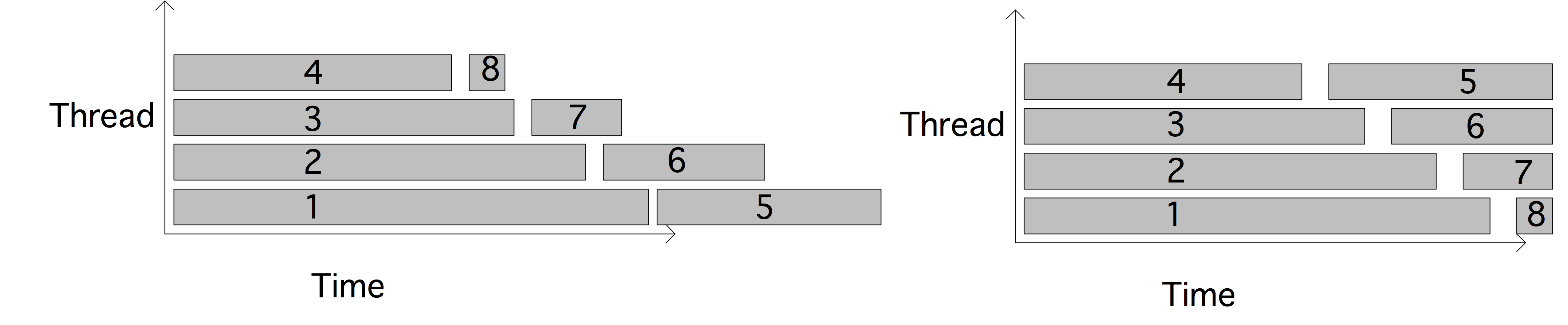
\caption{Static or round-robin (left) vs dynamic (right) thread scheduling; the task numbers are indicated.}

In static scheduling, the first thread gets tasks 1 and 4, the second 2 and 5, et cetera. In dynamic scheduling, any thread that finishes its task gets the next task. This clearly gives a better running time in this particular example. On the other hand, dynamic scheduling is likely to have a higher overhead.

2.10.3 Load balancing of independent tasks

crumb trail: > parallel > Load balancing > Load balancing of independent tasks

In other cases, work load is not directly determined by data. This can happen if there is a pool of work to be done, and the processing time for each work item is not easily computed from its description. In such cases we may want some flexibility in assigning work to processes.

Let us first consider the case of a job that can be partitioned into independent tasks that do not communicate. An example would be computing the pixels of a Mandelbrot set picture, where each pixel is set according to a mathematical function that does not depend on surrounding pixels. If we could predict the time it would take to draw an arbitrary part of the picture, we could make a perfect division of the work and assign it to the processors. This is known as static load balancing

More realistically, we can not predict the running time of a part of the job perfectly, and we use an overdecomposition of the work: we divide the work in more tasks than there are processors. These tasks are then assigned to a work pool  , and processors take the next job from the pool whenever they finish a balancing}. Many graph and combinatorial problems can be approached this way; see section  2.5.3  . For task assignment in a multicore context, see section  6.11  .

There are results that show that randomized assignment of tasks to processors is statistically close to optimal  [KarpZhang88]  , but this ignores the aspect that in scientific computing tasks typically communicate frequently.

Exercise Suppose you have tasks $\{T_i\}_{i=1,\ldots,N}$ with running times $t_i$, and an unlimited number of processors. Look up Brent's theorem in section  2.2.4  , and derive from it that the fastest execution scheme for the tasks can be characterized as follows: there is one processor that only executes the task with maximal $t_i$ value. (This exercise was inspired by  [Pospiech2015]  .)
End of exercise

2.10.4 Load balancing as graph problem

crumb trail: > parallel > Load balancing > Load balancing as graph problem

Next let us consider a parallel job where the parts do communicate. In this case we need to balance both the scalar workload and the communication.

A parallel computation can be formulated as a graph (see Appendix  app:graph for an introduction to graph theory) where the processors are the vertices, and there is an edge between two vertices if their processors need to communicate at some point. Such a graph is often derived from an underlying graph of the problem being solved. As an example consider the matrix-vector product $y=Ax$ where $A$ is a sparse matrix, and look in detail at the processor that is computing $y_i$ for some $i$. The statement $y_i\leftarrow y_i+A_{ij}x_j$ implies that this processor will need the value $x_j$, so, if this variable is on a different processor, it needs to be sent over.

We can formalize this: Let the vectors $x$ and $y$ be distributed disjointly over the processors, and define uniquely $P(i)$ as the processor that owns index $i$. Then there is an edge $(P,Q)$ if there is a nonzero element $a_{ij}$ with $P=P(i)$ and $Q=P(j)$. This graph is undirected in the case of a structurally symmetric matrix  , that is $a_{ij}\not=0\Leftrightarrow a_{ji}\not=0$.

The distribution of indices over the processors now gives us vertex and edge weights: a processor has a vertex weight that is the number of indices owned by it; an edge $(P,Q)$ has a weight that is the number of vector components that need to be sent from $Q$ to $P$, as described above.

The load balancing problem can now be formulated as follows:

Find a partitioning $\bbP=\cup_i \bbP_i$, such the variation in vertex weights is minimal, and simultaneously the edge weights are as low as possible.

Minimizing the variety in vertex weights implies that all processor have approximately the same amount of work. Keeping the edge weights low means that the amount of communication is low. These two objectives need not be satisfiable at the same time: some trade-off is likely.

Exercise Consider the limit case where processors are infinitely fast and bandwidth between processors is also unlimited. What is the sole remaining factor determining the runtime? What graph problem do you need to solve now to find the optimal load balance? What property of a sparse matrix gives the worst case behavior?
End of exercise

An interesting approach to load balancing comes from spectral graph theory (section  19.6  ): if $A_G$ is the adjacency matrix of an undirected graph and $D_G-A_G$ the graph Laplacian  , then the eigenvector $u_1$ to the smallest eigenvalue zero is positive, and the eigenvector $u_2$ to the next eigenvalue is orthogonal to it. Therefore $u_2$ has to have elements of alternating sign; further analysis shows that the elements with positive sign are connected, as are the negative ones. This leads to a natural bisection of the graph.

2.10.5 Load redistributing

crumb trail: > parallel > Load balancing > Load redistributing

In certain applications an initial load distribution is clear, but later adjustments are needed. A typical example is in FEM codes, where load can be distributed by a partitioning of the physical domain; see section  6.5.3  . If later the discretization of the domain changes, the load has to be rebalanced redistributed subsections we will see techniques for load balancing and rebalancing aimed at preserving locality.

2.10.5.1 Diffusion load balancing

crumb trail: > parallel > Load balancing > Load redistributing > Diffusion load balancing

In many practical situations we can associate a processor graph with our problem: there is a vertex between any pair of processes that directly interacts through point-to-point communication. Thus, it seems a natural thought to use this graph in load balancing, and only move load from a processor to its neighbors in the graph.

This is the idea by diffusion balancing  [Cybenko:1989:balancing,HuBlake:diffusion1999]  .

While the graph is not intrinsically directed, for load balancing we put arbitrary directions on the edges. Load balancing is then described as follows.

Let $\ell_i$ be the load on process $i$, and $\tau^{(j)}_i$ the transfer of load on an edge $j\rightarrow i$. Then \begin{equation} \ell_i \leftarrow \ell_i + \sum_{j\rightarrow i} \tau^{(j)}_i - \sum_{i\rightarrow j} \tau^{(i)}_j \end{equation} Although we just used a $i,j$ number of edges, in practice we put a linear numbering the edges. We then get a system \begin{equation} AT=\bar L \end{equation} where

• $A$ is a matrix of size $|N|\times|E|$ describing what edges connect in/out of a node, with elements values equal to $\pm1$ depending;
• $T$ is the vector of transfers, of size $|E|$; and
• $\bar L$ is the load deviation vector, indicating for each node how far over/under the average load they are.

In the case of a linear processor array this matrix is under-determined, with fewer edges than processors, but in most cases the system will be over-determined, with more edges than processes. Consequently, we solve \begin{equation} T= (A^tA)\inv A^t\bar L \qquad\hbox{or} T=A^t(AA^t)\inv \bar L. \end{equation} Since $A^tA$ and $AA^t$ are positive indefinite, we could solve the approximately by relaxation, needing only local knowledge. Of course, such relaxation has slow convergence, and a global method, such as CG  , would be faster  [HuBlake:diffusion1999]  .

2.10.5.2 Load balancing with space-filling curves

crumb trail: > parallel > Load balancing > Load redistributing > Load balancing with space-filling curves

In the previous sections we considered two aspects of load balancing: making sure all processors have an approximately equal amount of work, and letting the distribution reflect the structure of the problem so that communication is kept within reason. We can phrase the second point trying to preserve the locality of the problem when distributed over a parallel machine: points in space that are close together are likely to interact, so they should be on the same processor, or at least one not too far away.

Striving to preserve locality is not obviously the right strategy. In BSP (see section  2.6.8  ) a statistical argument is made that random placement will give a good load balance as well as balance of communication.

Exercise Consider the assignment of processes to processors, where the structure of the problem is such that each processes only communicates with its nearest neighbors, and let processors be ordered in a two-dimensional grid. If we do the obvious assignment of the process grid to the processor grid, there will be no contention. Now write a program that assigns processes to random processors, and evaluate how much contention there will be.
End of exercise

In the previous section you saw how graph partitioning techniques can help with the second point of preserving problem locality. In this section you will see a different technique that is attractive both for the initial load assignment and for subsequent load rebalancing  . In the latter case, a processor's work may increase or decrease, necessitating moving some of the load to a different processor.

For instance, some problems are adaptively refined

(Note: {For a detailed discussion, see  [Campbell:octree]  .}  )

 . This is illustrated in figure  2.31  .

FIGURE 2.31: Adaptive refinement of a domain in subsequent levels.

If we keep track of these refinement levels, the problem gets a tree structure, where the leaves contain all the work. Load balancing becomes a matter of partitioning the leaves of the tree over the processors; figure  2.32  .

FIGURE 2.32: Load distribution of an adaptively refined domain.

Now we observe that the problem has a certain locality: the subtrees of any non-leaf node are physically close, so there will probably be communication between them.

• Likely there will be more subdomains than processors; to minimize communication between processors, we want each processor to contain a simply connected group of subdomains. Moreover, we want each processor to cover a part of the domain that is `compact' in the sense that it has low aspect ratio, and low surface-to-volume ratio.
• When a subdomain gets further subdivided, part of the load of its processor may need to be shifted to another processor. This process of load redistributing should preserve locality.

To fulfill these requirements we use SFCs  . A SFC for the load balanced tree is shown in figure  2.33  . We will not give a formal discussion of SFCs ; instead we

FIGURE 2.33: A space filling curve for the load balanced tree.

will let figure  2.34 stand for a definition: a SFC is a recursively defined curve that touches each subdomain once

(Note: { SFCs were introduced by Peano as a mathematical device for constructing a continuous surjective function from the line segment $[0,1]$ to a higher dimensional cube $[0,1]^d$. This upset the intuitive notion of dimension that `you can not stretch and fold a line segment to fill up the square'. A proper treatment of the concept of dimension was later given by Brouwer.}  )

 .

FIGURE 2.34: Space filling curves, regularly and irregularly refined.

The SFC has the property that domain elements that are close together physically will be close together on the curve, so if we map the SFC to a linear ordering of processors we will preserve the locality of the problem.

More importantly, if the domain is refined by another level, we can refine the curve accordingly. Load can then be redistributed to neighboring processors on the curve, and we will still have locality preserved.

(The use of SFCs is N-body problems was discussed in  [Warren:1993:hash-octree] and  [Springel:gadget]  .)

2.11 Remaining topics

crumb trail: > parallel > Remaining topics

2.11.1 Distributed computing, grid computing, cloud computing

crumb trail: > parallel > Remaining topics > Distributed computing, grid computing, cloud computing

\SetBaseLevel 2

In this section we will take a short look at terms such as cloud computing and an earlier term distributed computing These are concepts that have a relation to parallel computing in the scientific sense, but that differ in certain fundamental ways.

Distributed computing can be traced back as coming from large database servers, such as airline reservations systems, which had to be accessed by many travel agents simultaneously. For a large enough volume of database accesses a single server will not suffice, so the mechanism of remote procedure call was invented, where the central server would call code (the procedure in question) on a different (remote) machine. The remote call could involve transfer of data, the data could be already on the remote machine, or there would be some mechanism that data on the two machines would stay synchronized. This gave rise to the SAN  . A generation later than distributed database systems, web servers had to deal with the same problem of many simultaneous accesses to what had to act like a single server.

We already see one big difference between distributed computing and high performance parallel computing. Scientific computing needs parallelism because a single simulation becomes too big or slow for one machine; the business applications sketched above deal with many users executing small programs (that is, database or web queries) against a large data set. For scientific needs, the processors of a parallel machine (the nodes in a cluster) have to have a very fast connection to each other; for business needs no such network is needed, as long as the central dataset stays coherent.

Both in HPC and in business computing, the server has to stay available and operative, but in distributed computing there is considerably more liberty in how to realize this. For a user connecting to a service such as a database, it does not matter what actual server executes their request. Therefore, distributed computing can make use of virtualization : a virtual server can be spawned off on any piece of hardware.

An analogy can be made between remote servers, which supply computing power wherever it is needed, and the electric grid, which supplies electric power wherever it is needed. This has led to \indexterm{grid computing} or utility computing  , with the Teragrid, owned by the US National Science Foundation, as an example. Grid computing was originally intended as a way of hooking up computers connected by a LAN or WAN  , often the Internet. The machines could be parallel themselves, and were often owned by different institutions. More recently, it has been viewed as a way of sharing resources, both datasets, software resources, and scientific instruments, over the network.

The notion of utility computing as a way of making services available, which you recognize from the above description of distributed computing, went mainstream with Google's search engine, which indexes the whole of the Internet. Another example is the GPS capability of Android mobile phones, which combines GIS, GPS, and mashup data. The computing model by which Google's gathers and processes data has been formalized in MapReduce  [Google:mapreduce]  . It combines a data parallel aspect (the `map' part) and a central accumulation part (`reduce'). Neither involves the tightly coupled neighbor-to-neighbor communication that is common in scientific computing. An open source framework for MapReduce computing exists in Hadoop  [Hadoop-wiki]  . Amazon offers a commercial Hadoop service.

The concept of having a remote computer serve user needs is attractive even if no large datasets are involved, since it absolves the user from the need of maintaining software on their local machine. Thus, Google Docs offers various `office' applications without the user actually installing any software. This idea is sometimes called SAS  , where the user connects to an `application server', and accesses it through a client such as a web browser. In the case of Google Docs, there is no longer a large central dataset, but each user interacts with their own data, maintained on Google's servers. This of course has the large advantage that the data is available from anywhere the user has access to a web browser.

The SAS concept has several connections to earlier technologies. For instance, after the mainframe and workstation eras, the so-called thin client idea was briefly popular. Here, the user would have a workstation rather than a terminal, yet work on data stored on a central server. One product along these lines was Sun's Sun Ray (circa 1999) where users relied on a smartcard to establish their local environment on an arbitrary, otherwise stateless, workstation.

2.11.2 Usage scenarios

crumb trail: > parallel > Remaining topics > Usage scenarios

The model where services are available on demand is attractive for businesses, which increasingly are using cloud services. The advantages are that it requires no initial monetary and time investment, and that no decisions about type and size of equipment have to be made. At the moment, cloud services are mostly focused on databases and office applications, but scientific clouds with a high performance interconnect are under development.

The following is a broad classification of usage scenarios of cloud resources

(Note: {Based on a blog post by Ricky Ho:

http://blogs.globallogic.com/five-cloud-computing-patterns  .}  )

 .

• Scaling. Here the cloud resources are used as a platform that can be expanded based on user demand. This can be considered Platform-as-a-Service (PAS): the cloud provides software and development platforms, eliminating the administration and maintenance for the user.

  We can distinguish between two cases: if the user is running single jobs and is actively waiting for the output, resources can be added to minimize the wait time for these jobs (capability computing). On the other hand, if the user is submitting jobs to a queue and the time-to-completion of any given job is not crucial (capacity computing), resources can be added as the queue grows.

  In HPC applications, users can consider the cloud resources as a cluster; this falls under Infrastructure-as-a-Service (IAS): the cloud service is a computing platforms allowing customization at the operating system level.

• Multi-tenancy. Here the same software is offered to multiple users, giving each the opportunity for individual customizations. This falls under Software-as-a-Service (SAS): software is provided on demand; the customer does not purchase software, but only pays for its use.
• Batch processing. This is a limited version of one of the Scaling scenarios above: the user has a large amount of data to process in batch mode. The cloud then becomes a batch processor. This model is a good candidate for MapReduce computations; section  2.11.5  .
• Storage. Most cloud providers offer database services, so this model absolves the user from maintaining their own database, just like the Scaling and Batch processing models take away the user's concern with maintaining cluster hardware.
• Synchronization. This model is popular for commercial user applications. Netflix and Amazon's Kindle allow users to consume online content (streaming movies and ebooks respectively); after pausing the content they can resume from any other platform. Apple's recent iCloud provides synchronization for data in office applications, but unlike Google Docs the applications are not `in the cloud' but on the user machine.

The first Cloud to be publicly accessible was Amazon's Elastic Compute cloud (EC2), launched in 2006. EC2 offers a variety of different computing platforms and storage facilities. Nowadays more than a hundred companies provide cloud based services, well beyond the initial concept of computers-for-rent.

The infrastructure for cloud computing can be interesting from a computer science point of view, involving distributed file systems, scheduling, virtualization, and mechanisms for ensuring high reliability.

An interesting project, combining aspects of grid and cloud computing is the Canadian Advanced Network For Astronomical Research [canfar-lecture]  . Here large central datasets are being made available to astronomers as in a grid, together with compute resources to perform analysis on them, in a cloud-like manner. Interestingly, the cloud resources even take the form of user-configurable virtual clusters.

2.11.3 Characterization

crumb trail: > parallel > Remaining topics > Characterization

Summarizing

(Note: {The remainder of this section is based on the NIST definition of cloud computing  http://csrc.nist.gov/publications/nistpubs/800-145/SP800-145.pdf  .}  )

we have three cloud computing service models :

• [Software as a Service] The consumer runs the provider's application, typically through a thin client such as a browser; the consumer does not install or administer software. A good example is Google Docs
• [Platform as a Service] The service offered to the consumer is the capability to run applications developed by the consumer, who does not otherwise manage the processing platform or data storage involved.
• [Infrastructure as a Service] The provider offers to the consumer both the capability to run software, and to manage storage and networks. The consumer can be in charge of operating system choice and network components such as firewalls.

These can be deployed as follows:

• [Private cloud] The cloud infrastructure is managed by one organization for its own exclusive use.
• [Public cloud] The cloud infrastructure is managed for use by a broad customer base.

One could also define hybrid models such as community clouds.

The characteristics of cloud computing are then:

• [On-demand and self service] The consumer can quickly request services and change service levels, without requiring human interaction with the provider.
• [Rapid elasticity] The amount of storage or computing power appears to the consumer to be unlimited, subject only to budgeting constraints. Requesting extra facilities is fast, in some cases automatic.
• [Resource pooling] Virtualization mechanisms make a cloud appear like a single entity, regardless its underlying infrastructure. In some cases the cloud remembers the `state' of user access; for instance, Amazon's Kindle books allow one to read the same book on a PC, and a smartphone; the cloud-stored book `remembers' where the reader left off, regardless the platform.
• [Network access] Clouds are available through a variety of network mechanisms, from web browsers to dedicated portals.
• [Measured service] Cloud services are typically `metered', with the consumer paying for computing time, storage, and bandwidth.

\SetBaseLevel 1

2.11.4 Capability versus capacity computing

crumb trail: > parallel > Remaining topics > Capability versus capacity computing

Large parallel computers can be used in two different ways. In later chapters you will see how scientific problems can be scaled up almost arbitrarily. This means that with an increasing need for accuracy or scale, increasingly large computers are needed. The use of a whole machine for a single problem, with only time-to-solution as the measure of success, is known as capability computing  .

On the other hand, many problems need less than a whole supercomputer to solve, so typically a computing center will set up a machine so that it serves a continuous stream of user problems, each smaller than the full machine. In this mode, the measure of success is the sustained performance per unit cost. This is known as capacity computing  , and it requires a finely tuned job scheduling strategy.

A popular scheme is fair-share scheduling  , which tries to allocate resources equally between users, rather than between processes. This means that it will lower a user's priority if the user had recent jobs, and it will give higher priority to short or small jobs. Examples of schedulers on this principle are SGE and Slurm  .

Jobs can have dependencies, which makes scheduling harder. In fact, under many realistic conditions scheduling problems are NP-complete  , so in practice heuristics will be used. This topic, while interesting, is not further discussed in this book.

2.11.5 MapReduce

crumb trail: > parallel > Remaining topics > MapReduce

MapReduce [Google:mapreduce] is a programming model for certain parallel operations. One of its distinguishing characteristics is that it is implemented using functional programming  . The MapReduce model handles computations of the following form:

• For all available data, select items that satisfy a certain criterion;
• and emit a key-value pair for them. This is the mapping stage.
• Optionally there can be a combine/sort stage where all pairs with the same key value are grouped together.
• Then do a global reduction on the keys, yielding one or more of the corresponding values. This is the reduction stage.

We will now give a few examples of using MapReduce, and present the functional programming model that underlies the MapReduce abstraction.

2.11.5.1 Expressive power of the MapReduce model

crumb trail: > parallel > Remaining topics > MapReduce > Expressive power of the MapReduce model

The reduce part of the MapReduce model makes it a prime candidate for computing global statistics on a dataset. One example would be to count how many times each of a set of words appears in some set of documents. The function being mapped knows the set of words, and outputs for each document a pair of document name and a list with the occurrence counts of the words. The reduction then does a componentwise sum of the occurrence counts.

The combine stage of MapReduce makes it possible to transform data. An example is a `Reverse Web-Link Graph': the map function outputs target-source pairs for each link to a target URL found in a page named "source". The reduce function concatenates the list of all source URLs associated with a given target URL and emits the pair target-list(source).

A less obvious example is computing PageRank (section  9.4  ) with MapReduce. Here we use the fact that the PageRank computation relies on a distributed sparse matrix-vector product. Each web page corresponds to a column of the web matrix $W$; given a probability $p_j$ of being on page $j$, that page can then compute tuples $\langle i,w_{ij}p_j\rangle$. The combine stage of MapReduce then sums together $(Wp)_i=\sum_j w_{ij}p_j$.

Database operations can be implemented with MapReduce but since it has a relatively large latency, it is unlikely to be competitive with standalone databases, which are optimized for fast processing of a single query, rather than bulk statistics.

Sorting with MapReduce is considered in section  8.5.1  .

For other applications see

http://horicky.blogspot.com/2010/08/designing-algorithmis-for-map-reduce.html  .

2.11.5.2 Mapreduce software

crumb trail: > parallel > Remaining topics > MapReduce > Mapreduce software

The implementation of MapReduce by Google was released under the name Hadoop  . While it suited the Google model of single-stage reading and processing of data, it had considerable disadvantages for many other users:

• Hadoop would flush all its data back to disc after each MapReduce cycle, so for operations that take more than a single cycle the file system and bandwidth demands are too great.
• In computing center environments, where a user's data is not continuously online, the time required for loading data into HDFS would likely overwhelm the actual analysis.

For these reasons, further projects such as Apache Spark ( https://spark.apache.org/  ) offer caching of data.

2.11.5.3 Implementation issues

crumb trail: > parallel > Remaining topics > MapReduce > Implementation issues

Implementing MapReduce on a distributed system has an interesting problem: the set of keys in the key-value pairs is dynamically determined. For instance, in the `word count' type of applications above we do not \textsl{a priori} know the set of words. Therefore it is not clear which reducer process to send the pair to.

We could for instance use a hash function to determine this. Since every process uses the same function, there is not disagreement. This leaves the problem that a process does not know how many messages with key-value pairs to receive. The solution to this was described in section  6.5.6  .

2.11.5.4 Functional programming

crumb trail: > parallel > Remaining topics > MapReduce > Functional programming

The mapping and reduction operations are readily implemented on any type of parallel architecture, using a combination of threading and message passing. However, at Google where this model was developed traditional parallelism was not attractive for two reasons. First of all, processors could fail during the computation, so a traditional model of parallelism would have to be enhanced with \indexterm{fault tolerance} mechanisms. Secondly, the computing hardware could already have a load, so parts of the computation may need to be migrated, and in general any type of synchronization between tasks would be very hard.

MapReduce is one way to abstract from such details of parallel computing, namely through adopting a functional programming model. In such a model the only operation is the evaluation of a function, applied to some arguments, where the arguments are themselves the result of a function application, and the result of the computation is again used as argument for another function application. In particular, in a strict functional model there are no variables, so there is no static data.

A function application, written in Lisp style as \n{(f a b)} (meaning that the function f is applied to arguments a and b  ) would then be executed by collecting the inputs from whereven they are to the processor that evaluates the function  f  . The mapping stage of a MapReduce process is denoted

  (map f (some list of arguments))

and the result is a list of the function results of applying f to the input list. All details of parallelism and of guaranteeing that the computation successfully finishes are handled by the map function.

Now we are only missing the reduction stage, which is just as simple:

(reduce g (map f (the list of inputs)))

The reduce function takes a list of inputs and performs a reduction on it.

The attractiveness of this functional model lies in the fact that functions can not have side effects : because they can only yield a single output result, they can not change their environment, and hence there is no coordination problem of multiple tasks accessing the same data.

Thus, MapReduce is a useful abstraction for programmers dealing with large amounts of data. Of course, on an implementation level the MapReduce software uses familiar concepts such as decomposing the data space, keeping a work list, assigning tasks to processors, retrying failed operations, et cetera.

2.11.6 The top500 list

crumb trail: > parallel > Remaining topics > The top500 list

There are several informal ways of measuring just `how big' a computer is. The most popular is the TOP500 list, maintained at

http://www.top500.org/  , which records a computer's performance on the Linpack benchmark  . Linpack is a package for linear algebra operations, and no longer in use, since it has been superseded by Lapack for shared memory and Scalapack for distributed memory computers. The benchmark operation is the solution of a (square, nonsingular, dense) linear system through LU factorization with partial pivoting, with subsequent forward and backward solution.

The LU factorization operation is one that has great opportunity for cache reuse, since it is based on the matrix-matrix multiplication kernel discussed in section  1.6.1  . It also has the property that the amount of work outweighs the amount of communication: $O(n^3)$ versus $O(n^2)$. As a result, the Linpack benchmark is likely to run at a substantial fraction of the peak speed of the machine. Another way of phrasing this is to say that the Linpack benchmark is a CPU-bound or compute-bound algorithm.

Typical efficiency figures are between 60 and 90 percent. However, it should be noted that many scientific codes do not feature the dense linear solution kernel, so the performance on this benchmark is not indicative of the performance on a typical code. Linear system solution through iterative methods (section  5.5  ), for instance, is much less efficient in a flops-per-second sense, being dominated by the bandwidth between CPU and memory (a  bandwidth-bound algorithm).

One implementation of the Linpack benchmark that is often used is `High-Performance LINPACK' ( http://www.netlib.org/benchmark/hpl/  ), which has several parameters such as blocksize that can be chosen to tune the performance.

2.11.6.1 The top500 list as a recent history of supercomputing

crumb trail: > parallel > Remaining topics > The top500 list > The top500 list as a recent history of supercomputing

The top500 list offers a history of almost 20 years of supercomputing. In this section we will take a brief look at historical developments

(Note: {The graphs contain John McCalpin's analysis of the top500 data.}  )

 . First of all, figure  2.35 shows the evolution of architecture types

FIGURE 2.35: Evolution of the architecture types on the top500 list.

by charting what portion of the aggregate peak performance of the whole list is due to each type.

• Vector machines feature a relatively small number of very powerful vector pipeline processors (section  2.3.1.1  ). This type of architecture has largely disappeared; the last major machine of this type was the Japanese Earth Simulator which is seen as the spike in the graph around 2002, and which was at the top of the list for two years.
• Micro-processor based architectures get their power from the large number of processors in one machine. The graph distinguishes between x86 ( Intel and AMD processors with the exception of the Intel Itanium  ) processors and others; see also the next graph.
• A number of systems were designed as highly scalable architectures: these are denoted MPP for `massively parallel processor'. In the early part of the timeline this includes architectures such as the Connection Machine  , later it is almost exclusively the IBM BlueGene  .
• In recent years `accelerated systems' are the upcoming trend. Here, a processing unit such as a GPU is attached to the networked main processor.

Next, figure  2.36 shows the dominance of the x86 processor type relative to other micro-processors.

FIGURE 2.36: Evolution of the architecture types on the top500 list.

(Since we classified the IBM BlueGene as an MPP, its processors are not in the `Power' category here.)

Finally, figure  2.37 shows the gradual increase in core count. Here we can make the following observations:

FIGURE 2.37: Evolution of the architecture types on the top500 list.

• In the 1990s many processors consisted of more than one chip. In the rest of the graph, we count the number of cores per `package', that is, per socket  . In some cases a socket can actually contain two separate dies.
• With the advent of multi-core processors, it is remarkable how close to vertical the section in the graph are. This means that new processor types are very quickly adopted, and the lower core counts equally quickly completely disappear.
• For accelerated systems (mostly systems with GPUs  ) the concept of `core count' is harder to define; the graph merely shows the increasing importance of this type of architecture.

2.11.7 Heterogeneous computing

crumb trail: > parallel > Remaining topics > Heterogeneous computing

You have now seen several computing models: single core, shared memory multicore, distributed memory clusters, GPUs. These models all have in common that, if there is more than one instruction stream active, all streams are interchangeable. With regard to GPUs we need to refine this statement: all instruction stream on the GPU are interchangeable. However, a GPU is not a standalone device, but can be considered a co-processor to a \indexterm{host processor}.

If we want to let the host perform useful work while the co-processor is active, we now have two different instruction streams or types of streams. This situation is known as heterogeneous computing  . In the GPU case, these instruction streams are even programmed by a slightly different mechanisms -- using CUDA for the GPU -- but this need not be the case: the Intel MIC architecture is programmed in ordinary C.