Sorting
Experimental html version of downloadable textbook, see https://theartofhpc.com
#1_1
vdots
#1_{#2-1} \end{pmatrix}} % {
left(
begin{array}{c} #1_0
#1_1
vdots
#1_{#2-1}
end{array}
right) } \] 8.1 : Brief introduction to sorting
8.1.1 : Complexity
8.1.2 : Sorting networks
8.1.3 : Parallel complexity
8.2 : Odd-even transposition sort
8.3 : Quicksort
8.3.1 : Quicksort in shared memory
8.3.2 : Quicksort on a hypercube
8.3.3 : Quicksort on a general parallel processor
8.4 : Radixsort
8.4.1 : Parallel radix sort
8.4.2 : Radix sort by most significant digit
8.5 : Samplesort
8.5.1 : Sorting through MapReduce
8.6 : Bitonic sort
Back to Table of Contents
8 Sorting
Sorting is not a common operation in scientific computing: one expects it to be more important in databases, whether these be financial or biological (for instance in sequence alignment). However, it sometimes comes up, for instance in AMR and other applications where significant manipulations of data structures occurs.
In this section we will briefly look at some basic algorithms and how they can be done in parallel. For more details, see [Kumar:parcomp-book] and the references therein.
8.1 Brief introduction to sorting
crumb trail: > sorting > Brief introduction to sorting
8.1.1 Complexity
crumb trail: > sorting > Brief introduction to sorting > Complexity
There are many sorting algorithms. Traditionally, they have been distinguished by their computational complexity, that is, given an array of $n$ elements, how many operations does it take to sort them, as a function of $n$.
Theoretically one can show that a sorting algorithm has to have at least complexity $O(n\log n)$\footnote{One can consider a sorting algorithm as a decision tree: a first comparison is made, depending on it two other comparisons are made, et cetera. Thus, an actual sorting becomes a path through this decision tree. If every path has running time $h$, the tree has $2^h$ nodes. Since a sequence of $n$ elements can be ordered in $n!$ ways, the tree needs to have enough paths to accomodate all of these; in other words, $2^h\geq n!$. Using Stirling's formula, this means that $n\geq O(n\log n)$}. There are indeed several algorithms that are guaranteed to attain this complexity, but a very popular algorithm, called Quicksort `expected' complexity of $O(n\log n)$, and a worst case complexity of $O(n^2)$. This behaviour results from the fact that quicksort needs to choose `pivot elements' (we will go into more detail below in section 8.3 ), and if these choices are consistently the worst possible, the optimal complexity is not reached.
\begin{displayalgorithm} \While{the input array has length $>1$}{ Find a pivot element of intermediate size\; Split the array in two, based on the pivot\; Sort the two arrays. }
MAIN 8.1: The quicksort algorithm.
\end{displayalgorithm}sort} algorithm always has the same complexity, since it has a static structure:
\begin{displayalgorithm} \For{$\mathit{pass}$ from $1$ to $n-1$}{ \For{$e$ from 1 to $n-\mathit{pass}$}{ \If{elements $e$ and $e+1$ are ordered the wrong way}{exchange them} } }
MAIN 8.2: The bubble sort algorithm.
\end{displayalgorithm}It is easy to see that this algorithm has a complexity of $O(n^2)$: the inner loop does $t$ comparisons and up to $t$ exchanges. Summing this from $1$ to $n-1$ gives approximately $n^2/2$ comparisons and at most the same number of exchanges.
8.1.2 Sorting networks
crumb trail: > sorting > Brief introduction to sorting > Sorting networks
Above we saw that some sorting algorithms operate independently of the actual input data, and some make decisions based on that data. The former class is sometimes called sorting network . It can be considered as custom hardware that implements just one algorithm. The basic hardware element is the compare-and-swap element, which has two inputs and two outputs. For two inputs $x,y$ the outputs are $\max(x,y)$ and $\min(x,y)$.
In figure 8.3 we show buble sort, built up
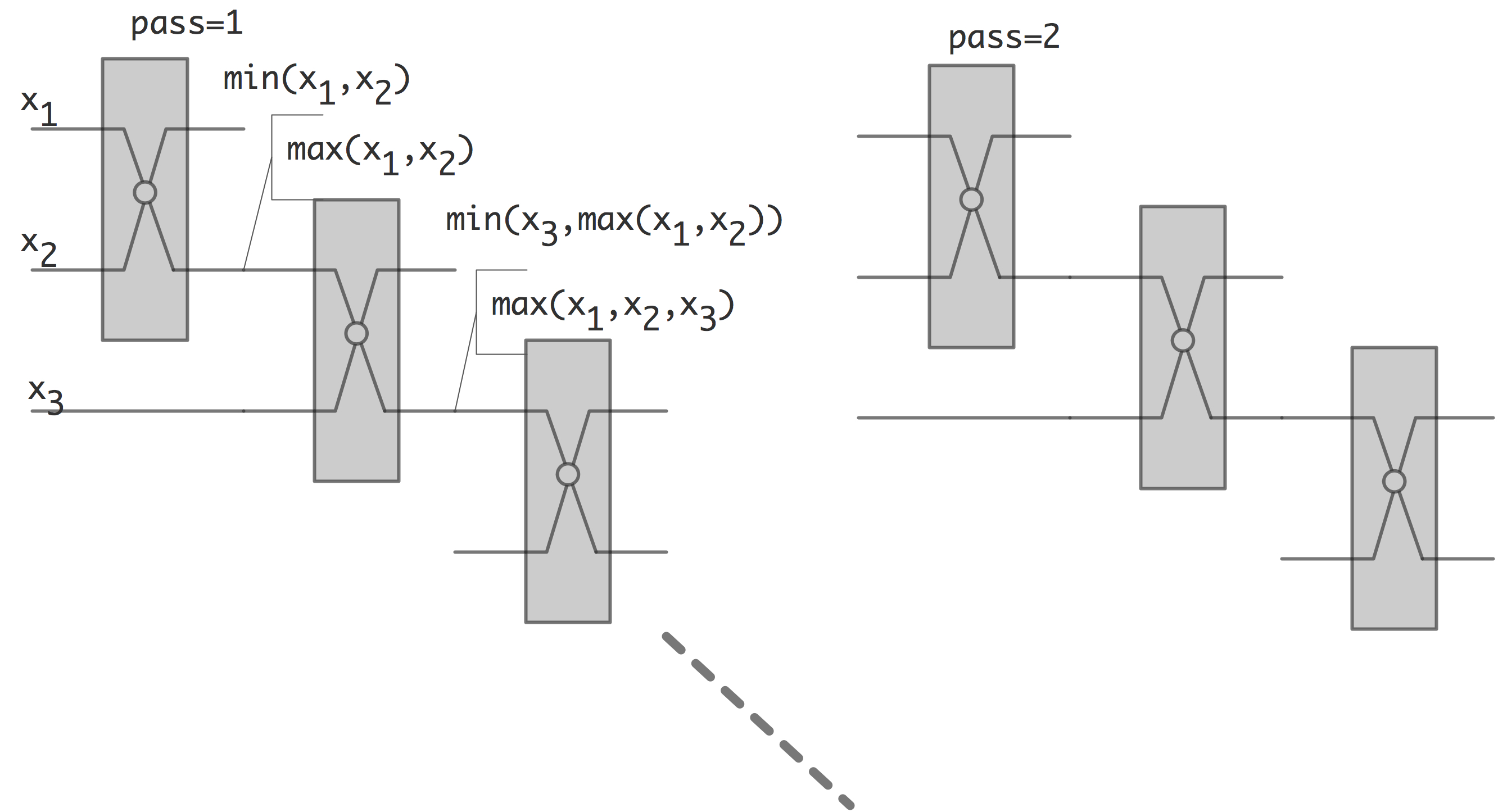
FIGURE 8.3: Bubble sort as a sorting network.
out of compare and swap elements.
Below we will consider the Bitonic sort algorithm as a prime example of a sorting network.
8.1.3 Parallel complexity
crumb trail: > sorting > Brief introduction to sorting > Parallel complexity
Above we remarked that sorting sequentially takes at least $O(N\log N)$ time. If we can have perfect speedup, using for simplicity $P=N$ processors, we would have parallel time $O(\log N)$. If the parallel time is more than that, we define the sequential complexity
as the total number of operations over all processors.
This equals the number of operations if the parallel algorithm were executed by one process, emulating all the others. Ideally this would be the same as the number of operations for a single-process algorithm, but it need not be. If it is larger, we have found another source of overhead: an intrinsic penalty for using a parallel algorithm. For instance, below we will see that sorting algorithm often have a sequential complexity of $O(N\log^2N)$.
odd-even transposition sort , \index{swap sort|see{odd-even transposition \index{exchange sort|see{odd-even transposition
8.2 Odd-even transposition sort
crumb trail: > sorting > Odd-even transposition sort
Taking another look at figure 8.3 , you see that the second pass
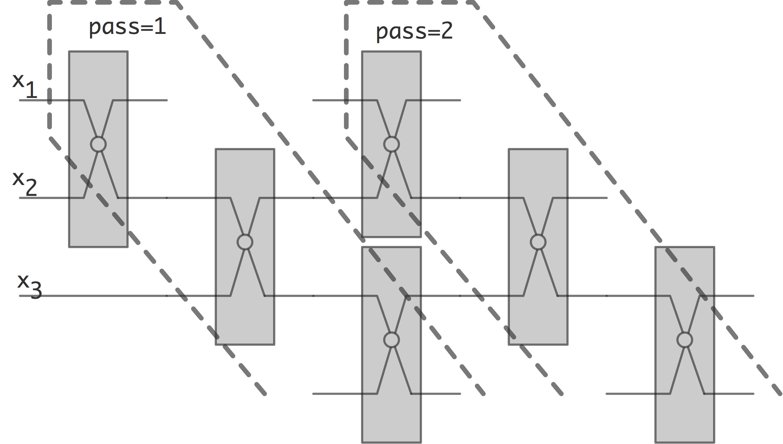
FIGURE 8.4: Overlapping passes in the bubble sort network.
can actually be started long before the first pass is totally finished. This is illustrated in figure 8.4 . If we now look at what happens at any given time, we obtain the odd-even transposition sort
Odd-even transposition sort is a simple parallel sorting algorithm, with as main virtue that it is relatively easy to implement on a linear area of processors. On the other hand, it is not particularly efficient.
A single step of the algorithm consists of two substeps:
-
Every even-numbered processor does a compare-and-swap with its right neighbour; then
-
Every odd-numbered processor does a compare-and-swap with its right neighbour.
Theorem
After $N/2$ steps, each consisting of the two substeps just given,
a sequency is sorted.
End of theorem
Proof
In each triplet $2i,2i+1,2i+2$, after an even and an odd step the
largest element will be in rightmost position. Proceed by induction.
End of proof
With a parallel time of $N$, this gives a sequential complexity $N^2$ compare-and-swap operations.
Exercise
Discuss speedup and efficiency of odd-even transposition sort sort, where we sort $N$ numbers of $P$ processors; for simplicity we set $N=P$ so that each processor contains a single number. Express execution time in compare-and-swap operations.
-
How many compare-and-swap operations does the parallel code take in total?
-
How many sequential steps does the algorithm take? What are $T_1$, $T_p$, $T_\infty$, $S_p$, $E_p$ for sorting $N$ numbers? What is the average amount of parallelism?
-
Odd-even transposition sort sort can be considered a parallel implementation of bubble sort. Now let $T_1$ refer to the execution time of (sequential) bubble sort. How does this change $S_p$ and $E_p$?
End of exercise
8.3 Quicksort
crumb trail: > sorting > Quicksort
Quicksort is a recursive algorithm, that, unlike bubble sort, is not deterministic. It is a two step procedure, based on a reordering of the sequence\footnote{The name is explained by its origin with the Dutch computer scientist Edsger Dijkstra; see
http://en.wikipedia.org/wiki/Dutch_national_flag_problem .}:
\begin{displayalgorithm} \TitleOfAlgo{Dutch National Flag ordering of an array} \Input{An array of elements, and a `pivot' value} \Output{The input array with elements ordered as red-white-blue, where red elements are larger than the pivot, white elements are equal to the pivot, and blue elements are less than the pivot} \end{displayalgorithm}
We state without proof that this can be done in $O(n)$ operations. With this, quicksort becomes:
\begin{displayalgorithm} \TitleOfAlgo{Quicksort} \Input{An array of elements} \Output{The input array, sorted} \While{The array is longer than one element}{ pick an arbitrary value as pivot \; apply the Dutch National Flag reordering to this array \; Quicksort( the blue elements ) \; Quicksort( the red elements ) \; } \end{displayalgorithm}
The indeterminacy of this algorithm, and the variance in its complexity, stems from the pivot choice. In the worst case, the pivot is always the (unique) smallest element of the array. There will then be no blue elements, the only white element is the pivot, and the recursive call will be on the array of $n-1$ red elements. It is easy to see that the running time will then be $O(n^2)$. On the other hand, if the pivot is always (close to) the median, that is, the element that is intermediate in size, then the recursive calls will have an about equal running time, and we get a recursive formula for the running time: \begin{equation} T_n = 2T_{n/2} + O(n) \end{equation} which is $O(n\log n)$; for proof, see section 14.2 .
We will now consider parallel implementations of quicksort.
8.3.1 Quicksort in shared memory
crumb trail: > sorting > Quicksort > Quicksort in shared memory
A simple parallelization of the quicksort algorithm can be achieved by executing the two recursive calls in parallel. This is easiest realized with a shared memory model, and threads (section 2.6.1 ) for the recursive calls.
function par_qs( data,nprocs ) {
  data_lo,data_hi = split(data);
  parallel do:
    par_qs( data_lo,nprocs/2 );
    par_qx( data_hi,nprocs/2 );
}
However, this implementation is not efficient without some effort. First of all, the recursion runs for $\log_2 n$ steps, and the amount of parallelism doubles in every step, so we could think that with $n$ processing elements the whole algorithm takes $\log_2 n$ time. However, this ignores that each step does not take a certain unit time. The problem lies in the splitting step which is not trivially parallel.
Exercise
Make this argument precise. What is the total running time, the
speedup, and the efficiency of parallelizing the quicksort algorithm
this way?
End of exercise
Is there a way to make splitting the array more efficient? As it turns out, yes, and the key is to use a parallel prefix operation ; see appendix app:prefix . If the array of values is $x_1,\ldots,x_n$, we use a parallel prefix to compute how many elements are less than the pivot $\pi$: \begin{equation} X_i=\#\{ x_j\colon j<i\wedge x_j<\pi \}. \end{equation} With this, if a processor looks at $x_i$, and $x_i$ is less than the pivot, it needs to be moved to location $X_i+1$ in the array where elements are split according to the pivot. Similarly, one would count how many elements there are over the pivot, and move those accordingly.
This shows that each pivoting step can be done in $O(\log n)$ time, and since there $\log n$ steps to the sorting algorithm, the total algorithm runs in $O((\log n)^2)$ time. The sequential complexity of quicksort
is $(\log_2N)^2$.
8.3.2 Quicksort on a hypercube
crumb trail: > sorting > Quicksort > Quicksort on a hypercube
As was apparent from the previous section, for an efficient parallelization of the quicksort algorithm, we need to make the Dutch National Flag reordering parallel too. Let us then assume that the array has been partitioned over the $p$ processors of a hypercube of dimension $d$ (meaning that $p=2^d$).
In the first step of the parallel algorithm, we choose a pivot, and broadcast it to all processors. All processors will then apply the reordering independently on their local data.
In order to bring together the red and blue elements in this first level, every processor is now paired up with one that has a binary address that is the same in every bit but the most significant one. In each pair, the blue elements are sent to the processor that has a 1 value in that bit; the red elements go to the processor that has a 0 value in that bit.
After this exchange (which is local, and therefore fully parallel), the processors with an address $1xxxxx$ have all the red elements, and the processors with an address $0xxxxx$ have all the blue elements. The previous steps can now be repeated on the subcubes.
This algorithm keeps all processors working in every step; however, it is susceptible to load imbalance if the chosen pivots are far from the median. Moreover, this load imbalance is not lessened during the sort process.
8.3.3 Quicksort on a general parallel processor
crumb trail: > sorting > Quicksort > Quicksort on a general parallel processor
Quicksort can also be done on any parallel machine that has a linear ordering of the processors. We assume at first that every processor holds exactly one array element, and, because of the flag reordering, sorting will always involve a consecutive set of processors.
Parallel quicksort of an array (or subarray in a recursive call) starts by constructing a binary tree on the processors storing the array. A pivot value is chosen and broadcast through the tree. The tree structure is then used to count on each processor how many elements in the left and right subtree are less than, equal to, or more than the pivot value.
With this information, the root processor can compute where the red/white/blue regions are going to be stored. This information is sent down the tree, and every subtree computes the target locations for the elements in its subtree.
If we ignore network contention, the reordering can now be done in unit time, since each processor sends at most one element. This means that each stage only takes time in summing the number of blue and red elements in the subtrees, which is $O(\log n)$ on the top level, $O(\log n/2)$ on the next, et cetera. This makes for almost perfect speedup.
8.4 Radixsort
crumb trail: > sorting > Radixsort
Most sorting algorithms are based on comparing the full item value. By contrast, radix sort does a number of partial sorting stages on the digits of the number. For each digit value a `bin' is allocated, and numbers are moved into these bins. Concatenating these bins gives a partially sorted array, and by moving through the digit positions, the array gets increasingly sorted.
Consider an example with number of at most two digits, so two stages are needed:
| \midrule array | 25 | 52 | 71 | 12 |
| \midrule last digit | 5 | 2 | 1 | 2 |
| (only bins 1,2,5 receive data) | ||||
| sorted | 71 | 52 | 12 | 25 |
| next digit | 7 | 5 | 1 | 2 |
| sorted | 12 | 25 | 52 | 71 |
| \midrule |
It is important that the partial ordering of one stage is preserved during the next. Inductively we then arrive at a totally sorted array in the end.
8.4.1 Parallel radix sort
crumb trail: > sorting > Radixsort > Parallel radix sort
A distributed memory sorting algorithm already has an obvious `binning' of the data, so a natural parallel implementation of radix sort is based on using $P$, the number of processes, as radix.
We illustrate this with an example on two processors, meaning that we look at binary representations of the values.
| \midrule | proc0 | proc0 | |||
| array | 2 | 5 | 7 | 1 | |
| binary | 010 | 101 | 111 | 001 | |
| \midrule stage 1: sort by least significant bit | |||||
| \midrule last digit | $\hphantom{00}0$ | $\hphantom{00}1$ | $\hphantom{00}1$ | $\hphantom{00}1$ | |
| (this serves as bin number) | |||||
| sorted | 010 | 101 | 111 | 001 | |
| \midrule stage 2: sort by middle bit | |||||
| \midrule next digit | $\hphantom{0}1 $ | $\hphantom{0}0 $ | $\hphantom{0}1 $ | $\hphantom{0}0$ | |
| (this serves as bin number) | |||||
| sorted | 101 | 001 | 010 | 111 | |
| \midrule stage 3: sort by most significant bit | |||||
| \midrule next digit | $\hphantom{}1 $ | $\hphantom{}0 $ | $\hphantom{}0 $ | $\hphantom{}1$ | |
| (this serves as bin number) | |||||
| sorted | 001 | 010 | 101 | 111 | |
| decimal | 1 | 2 | 5 | 7 | |
| \midrule |
(We see that there can be load imbalance during the algorithm.)
Analysis:
-
Determining the digits under consideration, and determining how many local values go into which bin are local operations. We can consider this as a connectivity matrix $C$ where $C[i,j]$ is the amount of data that process $i$ will send to process $j$. Each process owns its row of this matrix.
-
In order to receive data in the shuffle, each process needs to know how much data will receive from every other process. This requires a `transposition' of the connectivity matrix. In MPI terms, this is an
all-to-all operation: MPI_Alltoall .
-
After this, the actual data can be shuffled in another all-to-all operation. However, this the amounts differ per $i,j$ combination, we need the MPI_Alltoallv routine.
8.4.2 Radix sort by most significant digit
crumb trail: > sorting > Radixsort > Radix sort by most significant digit
It is perfectly possible to let the stages of the radix sort progress from most to least significant digit, rather than the reverse. Sequentially this does not change anything of significance.
However,
-
Rather than full shuffles, we are shuffling in increasingly small subsets, so even the sequential algorithm will have increased
spatial locality .
-
A shared memory parallel version will show similar locality improvements.
-
An MPI version no longer needs all-to-all operations. If we recognize that every next stage will be within a subset of processes, we can use the communicator splitting mechanism.
Exercise
The locality argument above was done somewhat hand-wavingly. Argue
that the algorithm can be done in both a
breadth-first
and
depth-first
fashion. Discuss the relation of this
distinction with the locality argument.
End of exercise
8.5 Samplesort
crumb trail: > sorting > Samplesort
You saw in Quicksort (section 8.3 ) that it is possible to use probabilistic elements in a sorting algorithm. We can extend the idea of picking a single pivot, as in Quicksort, to that of picking as many pivots as there are processors. Instead of a bisection of the elements, this divides the elements into as many `buckets' as there are processors. Each processor then sorts its elements fully in parallel.
\begin{displayalgorithm}
\Input{$p$: the number of processors, $N$: the numbers of elements to
sort; $\{x_i\}_{i MAIN 8.5: The Samplesort algorithm.
Clearly this algorithm can have severe load imbalance if the buckets are not chosen carefully. Randomly picking $p$ elements is probably not good enough; instead, some form of sampling of the elements is needed. Correspondingly, this algorithm is known as \textbf{Samplesort} [Blelloch:1991:CM2sort] .
While the sorting of the buckets, once assigned, is fully parallel, this algorithm still has some problems regarding parallelism. First of all, the sampling is a sequential bottleneck for the algorithm. Also, the step where buckets are assigned to processors is essentially an all-to-all operation,
For an analysis of this, assume that there are $P$ processes that first function as mappers, then as reducers. Let $N$ be the number of data points, and define a block size $b\equiv N/P$. The cost of the processing steps of the algorithm is:
-
The local determination of the bin for each element, which takes time $O(b)$; and
-
The local sort, for which is we can assume an optimal complexity of $b\log b$.
Exercise
Argue that for a small number of processes, $P\ll N$, this algorithm
has perfect speedup and a sequential complexity (see above) of
$N\log N$.
End of exercise
Comparing this algorithm to sorting networks like bitonic sort this sorting algorithm looks considerable simpler: it has only a one-step network. The previous question argued that in the `optimistic scaling' (work can increase while keeping number of processors constant) the sequential complexity is the same as for the sequential algorithm. However, in the weak scaling analysis where we increase work and processors proportionally, the sequential complexity is considerably worse.
Exercise
Consider the case where we scale both $N,P$, keeping $b$
constant.
Argue that in this case the shuffle step introduces an $N^2$ term
into the algorithm.
End of exercise
8.5.1 Sorting through MapReduce
crumb trail: > sorting > Samplesort > Sorting through MapReduce
The Terasort benchmark concerns sorting file-based dataset. Thus, it is somewhat of a standard in big data systems. In particular, MapReduce is a prime candidate; see
http://perspectives.mvdirona.com/2008/07/hadoop-wins-terasort/ .
Using MapReduce, the algorithm proceeds as follows:
-
A set of key values is determined through sampling or from prior information: the keys are such that an approximately equal number of records is expected to fall in between each pair. The number of intervals equals the number of reducer processes.
-
The mapper processes then produces key/value pairs where the key is the interval or reducer number.
-
The reducer processes then perform a local sort.
We see that, modulo terminology changes, this is really samplesort.
8.6 Bitonic sort
crumb trail: > sorting > Bitonic sort
To motivate bitonic sorting, suppose a sequence $x=\langle x_0,\ldots,x_n-1\rangle$ consists of an ascending followed by a descending part.
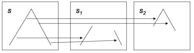
FIGURE 8.6: Illustration of a splitting a bitonic sequence.
Now split this sequence into two subsequences of equal length defined by: \begin{equation} \begin{array}{cc} s_1 = \langle \min\{x_0,x_{n/2}\},… \min\{ x_{n/2-1},x_{n-1}\}\\ s_2 = \langle \max\{x_0,x_{n/2}\},… \max\{ x_{n/2-1},x_{n-1}\}\\ \end{array} \label{eq:bitonic-split} \end{equation} From the picture it is easy to see that $s_1,s_2$ are again sequences with an ascending and descending part. Moreover, all the elements in $s_1$ are less than all the elements in $s_2$.8.6 second subsequence contains elements larger than in the first. Likewise we can construct a descending sorter by reversing the roles of maximum and minimum.
It's not hard to imagine that this is a step in a sorting algorithm: starting out with a sequence on this form, recursive application 8.6
FIGURE 8.7: Illustration of a bitonic network that sorts a bitonic sequence of length 16.
Figure 8.7 shows how 4 bitonic sorters, over distances 8,4,2,1 respectively, will sort a sequence of length 16.The actual definition of a bitonic sequence is slightly more complicated. A sequence is bitonic if it conists of an ascending part followed by a descending part, or is a cyclic permutation of such a sequence.
Exercise
Prove that splitting a bitonic sequence according to
8.6
End of exercise
So the question is how to get a bitonic sequence. The answer is to use larger and larger bitonic networks.
-
A bitonic sort of two elements gives you a sorted sequence.
-
If you have two sequences of length two, one sorted up, the other sorted down, that is a bitonic sequence.
-
So this sequence of length four can be sorted in two bitonic steps.
-
And two sorted sequences of length four form a bitonic sequence of length;
-
which can be sorted in three bitonic steps; et cetera.
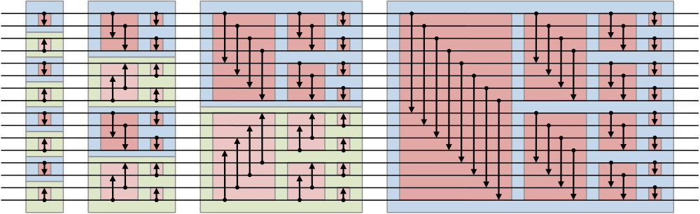
FIGURE 8.8: Full bitonic sort for 16 elements.
From this description you see that you $\log_2N$ stages to sort $N$ elements, where the $i$-th stage is of length $\log_2i$. This makes the total sequential complexity of bitonic sort $(\log_2N)^2$.
The sequence of operations in figure 8.8 is called a sorting network , built up out of simple compare-and-swap elements. There is no dependence on the value of the data elements, as is the case with quicksort.