\[ % mathjax inclusion. \newcommand\bbP{\mathbb{P}} \newcommand\bbR{\mathbb{R}} \newcommand\becomes{\mathop{:=}} \newcommand\dtdxx{\frac{\alpha\Delta t}{\Delta x^2}} \newcommand\defined{ \mathrel{\lower 5pt \hbox{${\equiv\atop\mathrm{\scriptstyle D}}$}}} \newcommand\fp[2]{#1\cdot10^{#2}} \newcommand\inv{^{-1}}\newcommand\invt{^{-t}} \newcommand\macro[1]{$\langle$#1$\rangle$} \newcommand\nobreak{} \newcommand\Rn{{\cal R}^n} \newcommand\Rnxn{{\cal R}^{n\times x}} \newcommand\sublocal{_{\mathrm\scriptstyle local}} \newcommand\toprule{\hline} \newcommand\midrule{\hline} \newcommand\bottomrule{\hline} \newcommand\multicolumn[3]{#3} \newcommand\defcolvector[2]{\begin{pmatrix} #1_0

#1_1


vdots

#1_{#2-1} \end{pmatrix}} % {
left(
begin{array}{c} #1_0

#1_1


vdots

#1_{#2-1}
end{array}
right) } \] 21.1 : Parallel prefix
21.2 : Sparse matrix vector product as parallel prefix
21.3 : Horner's rule
Back to Table of Contents

21 Parallel Prefix

For operations to be executable in parallel they need to be independent. That makes recurrences problematic to evaluate in parallel. Recurrences occur in obvious places such as solving a triangular system of equations (section  5.3.6  ), but they can also appear in sorting and many other operations.

In this appendix we look at parallel prefix operations: the parallel execution of an operation that is defined by a recurrence involving an associative operator. (See also section  6.9.2 for the `recursive doubling' approach to parallelizing recurrences.) Computing the sum of an array of elements is an example of this type of operation (disregarding the non-associativity

for the moment). Let $\pi(x,y)$ be the binary sum operator: \begin{equation} \pi(x,y)\equiv x+y, \end{equation} then we define the prefix sum of $n\geq 2$ terms as \begin{equation} \Pi(x_1,…,x_n) = \begin{cases} \pi(x_1,x_2)&\hbox{if $n=2$}\\ \pi\bigl( \Pi(x_1,…,x_{n-1}),x_n\bigr)&\hbox{otherwise} \\ \end{cases} \end{equation}

As a non-obvious example of a prefix operation, we could count the number of elements of an array that have a certain property.

Exercise Let $p(\cdot)$ be a predicate, $p(x)=1$ if it holds for $x$ and 0 otherwise. Define a binary operator $\pi(x,y)$ so that its reduction over an array of numbers yields the number of elements for which $p$ is true.
End of exercise

So let us now assume the existence of an associative operator $\oplus$, an array of values $x_1,\ldots,x_n$. Then we define the prefix problem as the computation of $X_1,\ldots,X_n$, where \begin{equation} \begin{cases} X_1=x_1\\ X_k=\oplus_{i\leq k} x_i \end{cases} \end{equation}

21.1 Parallel prefix

crumb trail: > prefix > Parallel prefix

The key to parallelizing the prefix problem is the realization that we can compute partial reductions in parallel: \begin{equation} x_1\oplus x_2, \quad x_3\oplus x_4, … \end{equation} are all independent. Furthermore, partial reductions of these reductions, \begin{equation} (x_1\oplus x_2) \oplus (x_3\oplus x_4),\quad … \end{equation} are also independent. We use the notation \begin{equation} X_{i,j}=x_i\oplus\cdots\oplus x_j \end{equation} for these partial reductions.

You have seen this before in section  2.1 : an array of $n$ numbers can be reduced in $\lceil \log_2 n\rceil$ steps. What is missing in the summation algorithm to make this a full prefix operation is computation of all intermediate values.

Observing that, for instance, $X_3=(x_1\oplus x_2)\oplus x_3=X_2\oplus x_3$, you can now imagine the whole process; see figure  21.1 for the case of $8$ elements.

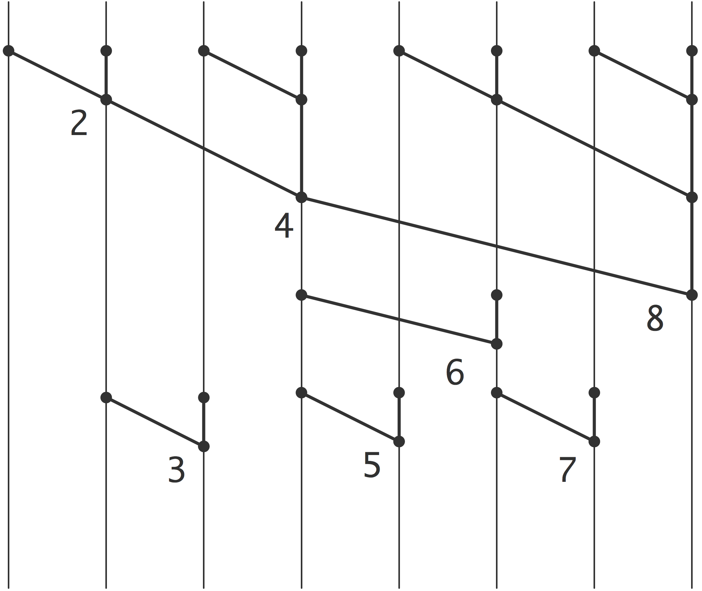
FIGURE 21.1: A prefix operation applied to 8 elements.

To compute, say, $X_{13}$, you express $13=8+4+1$ and compute $X_{13}=X_8\oplus X_{9,12} \oplus x_{13}$.

In this figure, operations over the same `distance' have been vertically aligned corresponding to a SIMD type execution. If the execution proceeds with a task graph, some steps can be executed earlier than the figure suggests; for instance $X_3$ can be computed simultaneously with $X_6$.

Regardless the arrangement of the computational steps, it is not hard to see that the whole prefix calculation can be done in $2\log_2n$ steps: $\log_2 n$ steps for computing the final reduction $X_n$, then another $\log_2 n$ steps for filling in the intermediate values.

21.2 Sparse matrix vector product as parallel prefix

crumb trail: > prefix > Sparse matrix vector product as parallel prefix

It has been observed that the sparse matrix vector product can be considered a prefix operation; see  [Blelloc:segmented-report]  . The reasoning here is we first compute all $y_{ij}\equiv a_{ij}x_j$, and subsequently compute the sums $y_i=\sum_j y_{ij}$ with a prefix operation.

A prefix sum as explained above does not compute the right result. The first couple of $y_{ij}$ terms do indeed sum to $y_1$, but then continuing the prefix sum gives $y_1+y_2$, instead of $y_2$. The trick to making this work is to consider two-component quantities $\langle y_{ij},s_{ij}\rangle$, where \begin{equation} s_{ij} = \begin{cases} 1&\hbox{if $j$ is the first nonzero index in row $i$}\\ 0&\hbox{otherwise} \end{cases} \end{equation} Now we can define prefix sums that are `reset' every time $s_{ij}=1$.

21.3 Horner's rule

crumb trail: > prefix > Horner's rule

Horner's rule for evaluating a polynomial is an example of a simple recurrence: \begin{equation} y = c_0 x^n +\cdots+ c_n x^0 \equiv \begin{cases} t_0 \leftarrow c_0\\ t_i \leftarrow t_{i-1}\cdot x + c_i&i=1,…,n\\ y = t_n\\ \end{cases} \end{equation} or, written more explicitly \begin{equation} y = \left(\left( ( c_0\cdot x + c_1 ) \cdot x + c_2 \right) \cdots \right) . \end{equation} Like many other recurrences, this seemingly sequential operation can be parallelized: \begin{equation} \begin{array}{cccc} c_0 x + c_1 & c_2 x + c_3 & c_4 x + c_5 & c_6 x + c_7\\ %% \multicolumn{2}{c}{${\upbracefill}$} & %% \multicolumn{2}{@{}c@{}}{${\upbracefill}$} \\ \multicolumn{2}{c}{\cdot \times x^2 + \cdot}& \multicolumn{2}{c}{\cdot \times x^2 + \cdot}\\ %% \multicolumn{4}{c}{${\upbracefill}$} \\ \multicolumn{4}{c}{\cdot \times x^4 + \cdot}\\ \end{array} \end{equation}

However, we see here that some cleverness is needed: we need $x,x^2,x^4$ etc.\ to multiply subresults.

Interpreting Horner's rule as a prefix scheme fails: the `horner operator' $h_x(a,b)=ax+b$ is easily seen not to be associative. From the above treewise calculation we see that we need to carry and update the $x$, rather than attaching it to the operator.

A little experimenting shows that \newcommand\xyvec[2]{ \left[

\begin{array}{c} #1

#2

\end{array} \right] } \begin{equation} h\left( \xyvec ax,\xyvec by \right) \equiv \xyvec {ay+b}{xy} \end{equation} serves our purposes: \begin{equation} h\left( \xyvec ax,\xyvec by ,\xyvec cz \right) = \left\{ \begin{array}{lll} h\left( h\left( \xyvec ax,\xyvec by \right ),\xyvec cz \right) &=& h\left( \xyvec {ay+b}{xy},\xyvec cz \right) \\ h\left( \xyvec ax,h\left( \xyvec by ,\xyvec cz \right ) \right) &=& h\left( \xyvec ax,\xyvec { bz+c } {yz} \right) \end{array} \right\} = \xyvec{ayz + bz +c}{xyz} \end{equation} With this we can realize Horner's rule as \begin{equation} h\left( \xyvec {c_0}x,\xyvec {c_1}x,…,\xyvec {c_n}x \right) \end{equation}

As an aside, this particular form of the `horner operator' corresponds to the `rho' operator in the programming language  APL  , which is normally phrased as evaluation in a number system with varying radix.