32 PETSc objects

32.1 Distributed objects

crumb trail: > petsc-objects > Distributed objects

PETSc is based on the SPMD model, and all its objects act like they exist in parallel, spread out over all the processes. Therefore, prior to discussing specific objects in detail, we briefly discuss how PETSc treats distributed objects.

For a matrix or vector you need to specify the size. This can be done two ways:

• you specify the global size and PETSc distributes the object over the processes, or
• you specify on each process the local size

For example, if you have a vector of $N$ components, or a matrix of $N$ rows, and you have $P$ processes, each process will receive $N/P$ components or rows if $P$ divides evenly in $N$. If $P$ does not divide evenly, the excess is spread over the processes.

The way the distribution is done is by contiguous blocks: with 10 processes and 1000 components in a vector, process 0 gets the range $0\cdots99$, process 1 gets $1\cdots199$, et cetera. This simple scheme suffices for many cases, but PETSc has facilities for more sophisticated load balancing.

32.1.1 Support for distributions

crumb trail: > petsc-objects > Distributed objects > Support for distributions

Once an object has been created and distributed, you do not need to remember the size or the distribution yourself: you can query these with calls such as \clstinline{VecGetSize}, \clstinline{VecGetLocalSize}.

The corresponding matrix routines \clstinline{MatGetSize}, \clstinline{MatGetLocalSize} give both information for the distributions in $i$ and $j$ direction, which can be independent. Since a matrix is distributed by rows, \clstinline{MatGetOwnershipRange} only gives a row range.

// split.c
N = 100; n = PETSC_DECIDE;
PetscSplitOwnership(comm,&n,&N);
PetscPrintf(comm,"Global %d, local %d\n",N,n);




N = PETSC_DECIDE; n = 10;
PetscSplitOwnership(comm,&n,&N);
PetscPrintf(comm,"Global %d, local %d\n",N,n);

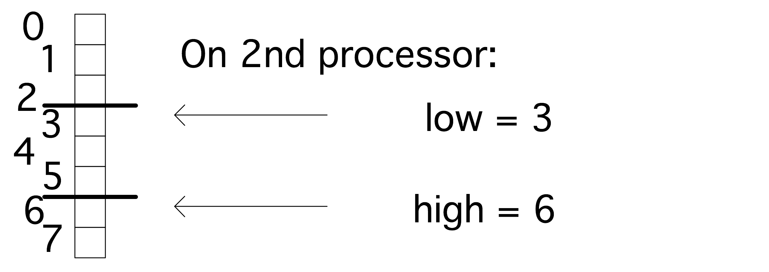
While PETSc objects are implemented using local memory on each process, conceptually they act like global objects, with a global indexing scheme. Thus, each process can query which elements out of the global object are stored locally. For vectors, the relevant routine is \clstinline{VecGetOwnershipRange}, which returns two parameters, \clstinline{low} and \clstinline{high}, respectively the first element index stored, and one-more-than-the-last index stored.

This gives the idiom:

VecGetOwnershipRange(myvector,&low,&high);
for (int myidx=low; myidx<high; myidx++)
  // do something at index myidx

These conversions between local and global size can also be done explicitly, using the PetscSplitOwnership routine. This routine takes two parameter, for the local and global size, and whichever one is initialized to PETSC_DECIDE gets computed from the other.

32.2 Scalars

crumb trail: > petsc-objects > Scalars

Unlike programming languages that explicitly distinguish between single and double precision numbers, PETSc has only a single scalar type: PetscScalar  . The precision of this is determined at installation time. In fact, a \clstinline{PetscScalar} can even be a complex number if the installation specified that the scalar type is complex.

Even in applications that use complex numbers there can be quantities that are real: for instance, the norm of a complex vector is a real number. For that reason, PETSc also has the type PetscReal  . There is also an explicit PetscComplex  .

Furthermore, there is

#define PETSC_BINARY_INT_SIZE    (32/8)
#define PETSC_BINARY_FLOAT_SIZE  (32/8)
#define PETSC_BINARY_CHAR_SIZE   (8/8)
#define PETSC_BINARY_SHORT_SIZE  (16/8)
#define PETSC_BINARY_DOUBLE_SIZE (64/8)
#define PETSC_BINARY_SCALAR_SIZE sizeof(PetscScalar)  

32.2.1 Integers

crumb trail: > petsc-objects > Scalars > Integers

Integers in PETSc are likewise of a size determined at installation time: PetscInt can be 32 or 64 bits. The latter possibility is useful for indexing into large vectors and matrices. Furthermore, there is a PetscErrorCode type for catching the return code of PETSc routines; see section  38.1.2  .

For compatibility with other packages there are two more integer types:

• PetscBLASInt is the integer type used by the BLAS  / LAPACK library. This is 32-bits if the -download-blas-lapack option is used, but it can be 64-bit if MKL is used. The routine PetscBLASIntCast casts a PetscInt to PetscBLASInt  , or returns PETSC_ERR_ARG_OUTOFRANGE if it is too large.
• PetscMPIInt is the integer type of the MPI library, which is always 32-bits. The routine PetscMPIIntCast casts a PetscInt to PetscMPIInt  , or returns PETSC_ERR_ARG_OUTOFRANGE if it is too large.

32.2.2 Complex

crumb trail: > petsc-objects > Scalars > Complex

Numbers of type PetscComplex have a precision matching PetscReal  .

Form a complex number using PETSC_i :

PetscComplex x = 1.0 + 2.0 * PETSC_i;

The real and imaginary part can be extract with the functions PetscRealPart and PetscImaginaryPart which return a PetscReal  .

There are also routines VecRealPart and VecImaginaryPart that replace a vector with its real or imaginary part respectively. Likewise MatRealPart and MatImaginaryPart  .

32.2.3 MPI Scalars

crumb trail: > petsc-objects > Scalars > MPI Scalars

For MPI calls, MPIU_REAL is the MPI type corresponding to the current PetscReal  .

For MPI calls, MPIU_SCALAR is the MPI type corresponding to the current PetscScalar  .

For MPI calls, MPIU_COMPLEX is the MPI type corresponding to the current PetscComplex  .

32.2.4 Booleans

crumb trail: > petsc-objects > Scalars > Booleans

There is a PetscBool datatype with values PETSC_TRUE and PETSC_FALSE  .

32.3 Vec: Vectors

crumb trail: > petsc-objects > Vec: Vectors

Vectors are objects with a linear index. The elements of a vector are floating point numbers or complex numbers (see section  32.2  ), but not integers: for that see section  32.5.1  .

32.3.1 Vector construction

crumb trail: > petsc-objects > Vec: Vectors > Vector construction

Constructing a vector takes a number of steps. First of all, the vector object needs to be created on a communicator with VecCreate

Python note In python, \plstinline{PETSc.Vec()} creates an object with null handle, so a subsequent \plstinline{create()} call is needed. In C and Fortran, the vector type is a keyword; in Python it is a member of PETSc.Vec.Type  .

## setvalues.py
comm = PETSc.COMM_WORLD
x = PETSc.Vec().create(comm=comm)
x.setType(PETSc.Vec.Type.MPI)

The corresponding routine VecDestroy deallocates data and zeros the pointer. (This and all other Destroy routines are collective because of underlying MPI technicalities.)

The vector type needs to be set with VecSetType  .

The most common vector types are:

• VECSEQ for sequential vectors, that is, living on a single process; This is typically created on the MPI_COMM_SELF or PETSC_COMM_SELF communicator.
• VECMPI for a vector distributed over the communicator. This is typically created on the MPI_COMM_WORLD or PETSC_COMM_WORLD communicator, or one derived from it.
• VECSTANDARD is VECSEQ when used on a single process, or VECMPI on multiple.

You may wonder why these types exist: you could have just one type, which would be as parallel as possible. The reason is that in a parallel run you may occasionally have a separate linear system on each process, which would require a sequential vector (and matrix) on each process, not part of a larger linear system.

Once you have created one vector, you can make more like it by VecDuplicate  ,

VecDuplicate(Vec old,Vec *new);

VecDuplicateVecs(Vec old,PetscInt n,Vec **new);

VecDestroyVecs(PetscInt n,Vec **vecs);

32.3.2 Vector layout

crumb trail: > petsc-objects > Vec: Vectors > Vector layout

Next in the creation process the vector size is set with VecSetSizes  . Since a vector is typically distributed, this involves the global size and the sizes on the processors. Setting both is redundant, so it is possible to specify one and let the other be computed by the library. This is indicated by setting it to PETSC_DECIDE  .

Python note Use \plstinline{PETSc.DECIDE} for the parameter not specified:

x.setSizes([2,PETSc.DECIDE])

The size is queried with VecGetSize for the global size and \indexpetscxref{VecGetLocalSize}{VecGetSize} for the local size.

Each processor gets a contiguous part of the vector. Use VecGetOwnershipRange to query the first index on this process, and the first one of the next process.

In general it is best to let PETSc take care of memory management of matrix and vector objects, including allocating and freeing the memory. However, in cases where PETSc interfaces to other applications it maybe desirable to create a \clstinline{Vec} object from an already allocated array: VecCreateSeqWithArray and VecCreateMPIWithArray  .

VecCreateSeqWithArray
   (MPI_Comm comm,PetscInt bs,
    PetscInt n,PetscScalar *array,Vec *V);
VecCreateMPIWithArray
   (MPI_Comm comm,PetscInt bs,
    PetscInt n,PetscInt N,PetscScalar *array,Vec *vv);  

As you will see in section  32.4.1  , you can also create vectors based on the layout of a matrix, using MatCreateVecs  .

32.3.3 Vector operations

crumb trail: > petsc-objects > Vec: Vectors > Vector operations

There are many routines operating on vectors that you need to write scientific applications. Examples are: norms, vector addition (including BLAS -type `AXPY' routines: VecAXPY  ), pointwise scaling, inner products. A large number of such operations are available in PETSc through single function calls to {VecXYZ} routines.

For debugging purpoases, the VecView routine can be used to display vectors on screen as ascii output,

// fftsine.c
PetscCall( VecView(signal,PETSC_VIEWER_STDOUT_WORLD) );
PetscCall( MatMult(transform,signal,frequencies) );
PetscCall( VecScale(frequencies,1./Nglobal) );
PetscCall( VecView(frequencies,PETSC_VIEWER_STDOUT_WORLD) );

Here are a couple of representative vector routines:

PetscReal lambda;
ierr = VecNorm(y,NORM_2,&lambda); CHKERRQ(ierr);
ierr = VecScale(y,1./lambda); CHKERRQ(ierr);  

Exercise Create a vector where the values are a single sine wave. using VecGetSize  , VecGetLocalSize  , VecGetOwnershipRange  . Quick visual inspection:

ibrun vec -n 12 -vec_view

Exercise Use the routines VecDot  , VecScale and VecNorm to compute the inner product of vectors x,y  , scale the vector  x  , and check its norm: \begin{equation} \begin{array}{l} p \leftarrow x^ty\\ x \leftarrow x/p\\ n \leftarrow \|x\|_2\\ \end{array} \end{equation}
End of exercise

Python note The plus operator is overloaded so that

    x+y

    x.sum() # max,min,....
    x.dot(y)
    x.norm(PETSc.NormType.NORM_INFINITY)

32.3.3.1 Split collectives

crumb trail: > petsc-objects > Vec: Vectors > Vector operations > Split collectives

MPI is capable (in principle) of `overlapping computation and communication', or latency hiding  . PETSc supports this by splitting norms and inner products into two phases.

• Start inner product / norm with VecDotBegin  / VecNormBegin ;
• Conclude inner product / norm with VecDotEnd  / VecNormEnd ;

32.3.4 Vector elements

crumb trail: > petsc-objects > Vec: Vectors > Vector elements

Setting elements of a traditional array is simple. Setting elements of a distributed array is harder. First of all, VecSet sets the vector to a constant value:

ierr = VecSet(x,1.); CHKERRQ(ierr);  

In the general case, setting elements in a PETSc vector is done through a function VecSetValue for setting elements that uses global numbering; any process can set any elements in the vector. There is also a routine VecSetValues for setting multiple elements. This is mostly useful for setting dense subblocks of a block matrix.

We illustrate both routines by setting a single element with VecSetValue  , and two elements with VecSetValues  . In the latter case we need an array of length two for both the indices and values. The indices need not be successive.

i = 1; v = 3.14;
VecSetValue(x,i,v,INSERT_VALUES);
ii[0] = 1; ii[1] = 2; vv[0] = 2.7; vv[1] = 3.1;
VecSetValues(x,2,ii,vv,INSERT_VALUES);

Fortran note The value/values routines work the same way in Fortran. Note that despite type checking, using the `values' routine and passing scalars, is allowed: End of Fortran note

Python note Single element:

x.setValue(0,1.)

x.setValues( [2*procno,2*procno+1], [2.,3.] )

Using \clstinline{VecSetValue} for specifying a local vector element corresponds to simple insertion in the local array. However, an element that belongs to another process needs to be transferred. This done in two calls: VecAssemblyBegin and VecAssemblyEnd  .

if (myrank==0) then
   do vecidx=0,globalsize-1
      vecelt = vecidx
      call VecSetValue(vector,vecidx,vecelt,INSERT_VALUES,ierr)
   end do
end if
call VecAssemblyBegin(vector,ierr)
call VecAssemblyEnd(vector,ierr)

(If you know the MPI library, you'll recognize that the first call corresponds to posting nonblocking send and receive calls; the second then contains the wait calls. Thus, the existence of these separate calls make latency hiding possible.)

VecAssemblyBegin(myvec);
// do work that does not need the vector myvec
VecAssemblyEnd(myvec);

Elements can either be inserted with INSERT_VALUES  , or added with ADD_VALUES in the VecSetValue  / VecSetValues call. You can not immediately mix these modes; to do so you need to call VecAssemblyBegin  / VecAssemblyEnd in between add/insert phases.

32.3.4.1 Explicit element access

crumb trail: > petsc-objects > Vec: Vectors > Vector elements > Explicit element access

Since the vector routines cover a large repertoire of operations, you hardly ever need to access the actual elements. Should you still need those elements, you can use VecGetArray for general access or \indexpetscxref{VecGetArrayRead}{VecGetArray} for read-only.

PETSc insists that you properly release this pointer again with VecRestoreArray or \indexpetscxref{VecRestoreArrayRead}{VecRestoreArray}.

In the following example, a vector is scaled through direct array access. Note the differing calls for the source and target vector, and note the const qualifier on the source array:

// vecarray.c
PetscScalar const *in_array;
PetscScalar *out_array;
VecGetArrayRead(x,&in_array);
VecGetArray(y,&out_array);
PetscInt localsize;
VecGetLocalSize(x,&localsize);
for (int i=0; i<localsize; i++)
  out_array[i] = 2*in_array[i];
VecRestoreArrayRead(x,&in_array);
VecRestoreArray(y,&out_array);

This example also uses VecGetLocalSize to determine the size of the data accessed. Even running in a distributed context you can only get the array of local elements. Accessing the elements from another process requires explicit communication; see section  32.5.2  .

There are some variants to the \clstinline{VecGetArray} operation:

• \indexpetscxref{VecReplaceArray}{VecPlaceArray} frees the memory of the \clstinline{Vec} object, and replaces it with a different array. That latter array needs to be allocated with PetscMalloc  .
• VecPlaceArray also installs a new array in the vector, but it keeps the original array; this can be restored with VecResetArray  .

Putting the array of one vector into another has a common application, where you have a distributed vector, but want to apply PETSc operations to its local section as if it were a sequential vector. In that case you would create a sequential vector, and VecPlaceArray the contents of the distributed vector into it.

Fortran note There are routines such as VecGetArrayF90 (with corresponding VecRestoreArrayF90  ) that return a (Fortran) pointer to a one-dimensional array.

!! vecset.F90
  Vec            :: vector
  PetscScalar,dimension(:),pointer :: elements
  call VecGetArrayF90(vector,elements,ierr)
  write (msg,10) myrank,elements(1)
10 format("First element on process",i3,":",f7.4,"\n")
  call PetscSynchronizedPrintf(comm,msg,ierr)
  call PetscSynchronizedFlush(comm,PETSC_STDOUT,ierr)
  call VecRestoreArrayF90(vector,elements,ierr)

!! vecarray.F90
  PetscScalar,dimension(:),Pointer :: &
       in_array,out_array
  call VecGetArrayReadF90( x,in_array,ierr )
  call VecGetArrayF90( y,out_array,ierr )
  call VecGetLocalSize( x,localsize,ierr )
  do index=1,localsize
     out_array(index) = 2*in_array(index)
  end do
  call VecRestoreArrayReadF90( x,in_array,ierr )
  call VecRestoreArrayF90( y,out_array,ierr )

Python note

    x.getArray()
    x.getValues(3)
    x.getValues([1, 2])

32.3.5 File I/O

crumb trail: > petsc-objects > Vec: Vectors > File I/O

As mentioned above, VecView can be used for displaying a vector on the terminal screen. However, viewers are actually much more general. As explained in section  38.2.2  , they can also be used to export vector data, for instance to file.

The converse operation, to load a vector that was exported in this manner, is VecLoad  .

Since these operations are each other's inverses, usually you don't need to know the file format. But just in case:

PetscInt    VEC_FILE_CLASSID
PetscInt    number of rows
PetscScalar *values of all entries

32.4 Mat: Matrices

crumb trail: > petsc-objects > Mat: Matrices

PETSc matrices come in a number of types, sparse and dense being the most important ones. Another possibility is to have the matrix in operation form, where only the action $y\leftarrow Ax$ is defined.

32.4.1 Matrix creation

crumb trail: > petsc-objects > Mat: Matrices > Matrix creation

Creating a matrix also starts by specifying a communicator on which the matrix lives collectively: MatCreate

Set the matrix type with MatSetType  . The main choices are between sequential versus distributed and dense versus sparse, giving types: MATMPIDENSE  , MATMPIAIJ  , MATSEQDENSE  , MATSEQAIJ  .

Distributed matrices are partitioned by block rows: each process stores a block row  , that is, a contiguous set of matrix rows. It stores all elements in that block row.

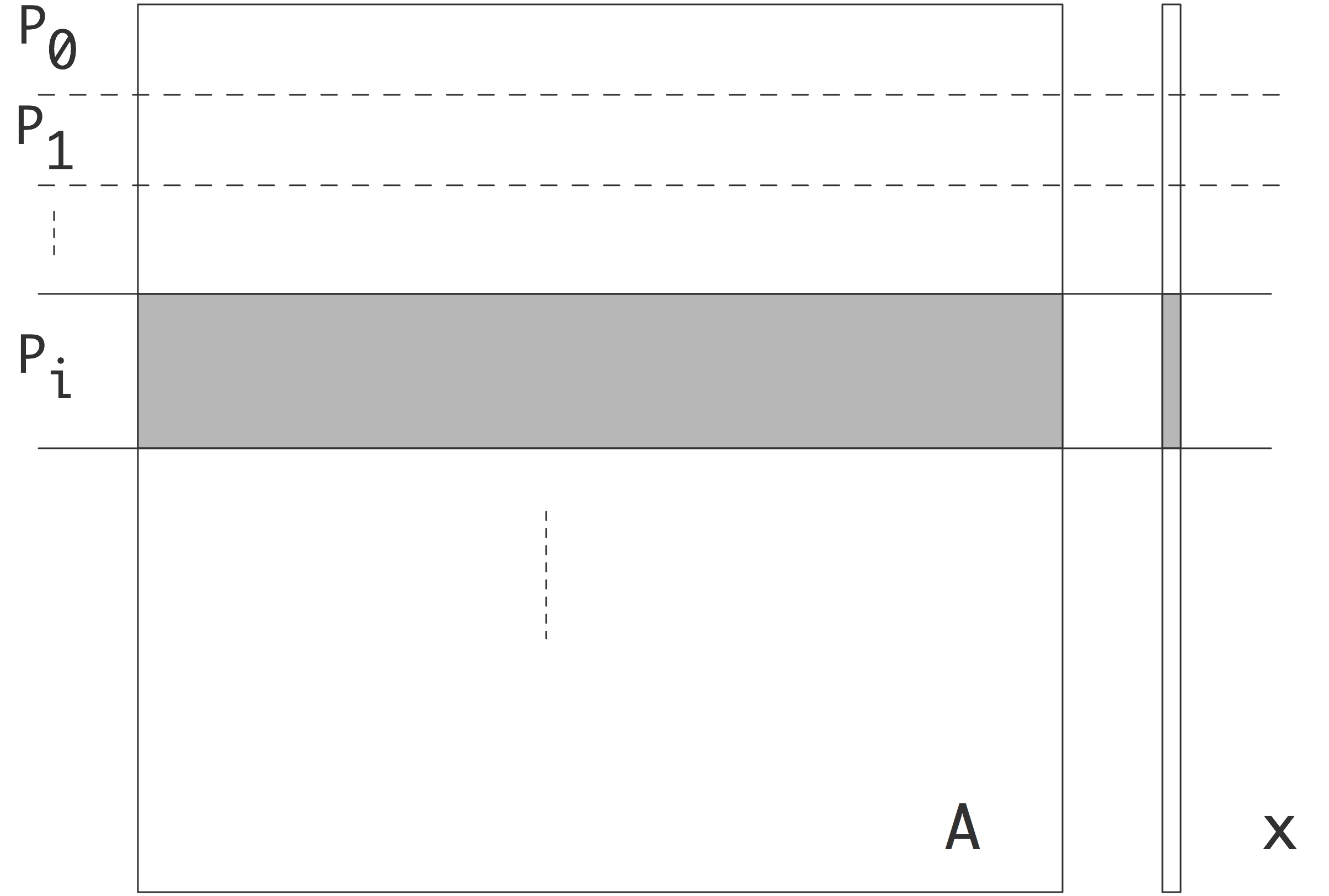
FIGURE 32.1: Matrix partitioning by block rows

In order for a matrix-vector product to be executable, both the input and output vector need to be partitioned conforming to the matrix.

While for dense matrices the block row scheme is not scalable, for matrices from PDEs it makes sense. There, a subdivision by matrix blocks would lead to many empty blocks.

Just as with vectors, there is a local and global size; except that that now applies to rows and columns. Set sizes with MatSetSizes and subsequently query them with MatSizes  . The concept of local column size is tricky: since a process stores a full block row you may expect the local column size to be the full matrix size, but that is not true. The exact definition will be discussed later, but for square matrices it is a safe strategy to let the local row and column size to be equal.

Instead of querying a matrix size and creating vectors accordingly, the routine MatCreateVecs can be used. (Sometimes this is even required; see section  32.4.9  .)

32.4.2 Nonzero structure

crumb trail: > petsc-objects > Mat: Matrices > Nonzero structure

In case of a dense matrix, once you have specified the size and the number of MPI processes, it is simple to determine how much space PETSc needs to allocate for the matrix. For a sparse matrix this is more complicated, since the matrix can be anywhere between completely empty and completely filled in. It would be possible to have a dynamic approach where, as elements are specified, the space grows; however, repeated allocations and re-allocations are inefficient. For this reason PETSc puts a small burden on the programmer: you need to specify a bound on how many elements the matrix will contain.

We explain this by looking at some cases. First we consider a matrix that only lives on a single process. You would then use MatSeqAIJSetPreallocation  . In the case of a tridiagonal matrix you would specify that each row has three elements:

MatSeqAIJSetPreallocation(A,3, NULL);

If the matrix is less regular you can use the third argument to give an array of explicit row lengths:

int *rowlengths;
// allocate, and then:
for (int row=0; row<nrows; row++)
  rowlengths[row] = // calculation of row length
MatSeqAIJSetPreallocation(A,NULL,rowlengths);

In case of a distributed matrix you need to specify this bound with respect to the block structure of the matrix. As illustrated in figure  32.2  , a matrix has a diagonal part and an off-diagonal part.

FIGURE 32.2: The diagonal and off-diagonal parts of a matrix

The diagonal part describes the matrix elements that couple elements of the input and output vector that live on this process. The off-diagonal part contains the matrix elements that are multiplied with elements not on this process, in order to compute elements that do live on this process.

The preallocation specification now has separate parameters for these diagonal and off-diagonal parts: with \indexpetscxref{MatMPIAIJSetPreallocation}{MatSeqAIJSetPreallocation}. you specify for both either a global upper bound on the number of nonzeros, or a detailed listing of row lengths. For the matrix of the Laplace equation  , this specification would seem to be:

MatMPIAIJSetPreallocation(A, 3, NULL, 2, NULL);

Specifying bounds on the number of nonzeros is often enough, and not too wasteful. However, if many rows have fewer nonzeros than these bounds, a lot of space is wasted. In that case you can replace the NULL arguments by an array that lists for each row the number of nonzeros in that row.

32.4.3 Matrix elements

crumb trail: > petsc-objects > Mat: Matrices > Matrix elements

You can set a single matrix element with MatSetValue or a block of them, where you supply a set of $i$ and $j$ indices, using MatSetValues  .

After setting matrix elements, the matrix needs to be assembled. This is where PETSc moves matrix elements to the right processor, if they were specified elsewhere. As with vectors this takes two calls: MatAssemblyBegin and \indexpetscxref{MatAssemblyEnd}{MatAssemblyBegin} which can be used to achieve latency hiding  .

Elements can either be inserted ( INSERT_VALUES  ) or added ( ADD_VALUES  ). You can not immediately mix these modes; to do so you need to call MatAssemblyBegin  / MatAssemblyEnd with a value of MAT_FLUSH_ASSEMBLY  .

PETSc sparse matrices are very flexible: you can create them empty and then start adding elements. However, this is very inefficient in execution since the OS needs to reallocate the matrix every time it grows a little. Therefore, PETSc has calls for the user to indicate how many elements the matrix will ultimately contain.

MatSetOption(A, MAT_NEW_NONZERO_ALLOCATION_ERR, PETSC_FALSE)

32.4.3.1 Element access

crumb trail: > petsc-objects > Mat: Matrices > Matrix elements > Element access

If you absolutely need access to the matrix elements, there are routines such as MatGetRow  . With this, any process can request, using global row numbering, the contents of a row that it owns. (Requesting elements that are not local requires the different mechanism of taking submatrices; section  32.4.6  .)

Since PETSc is geared towards sparse matrices this returns not only the element values, but also the column numbers, as well as the mere number of stored columns. If any of these three return values are not needed, they can be unrequested by setting the parameter passed to \clstinline{NULL}.

PETSc insists that you properly release the row again with \indexpetscxref{MatRestoreRow}{MatGetRow}.

It is also possible to retrieve the full CRS contents of the local matrix with MatDenseGetArray  , MatDenseRestoreArray  , MatSeqAIJGetArray  , MatSeqAIJRestoreArray  . (Routines \indexpetscdepr{MatGetArray} / \indexpetscdepr{MatRestoreArray} are deprecated.)

32.4.4 Matrix viewers

crumb trail: > petsc-objects > Mat: Matrices > Matrix viewers

Matrices can be `viewed' (see section  38.2.2 for a discussion of the PetscViewer mechanism) in a variety of ways, starting with the MatView call. However, often it is more convenient to use online options such as

yourprogram -mat_view
yourprogram -mat_view draw
yourprogram -ksp_mat_view draw

32.4.5 Matrix operations

crumb trail: > petsc-objects > Mat: Matrices > Matrix operations

32.4.5.1 Matrix-vector operations

crumb trail: > petsc-objects > Mat: Matrices > Matrix operations > Matrix-vector operations

In the typical application of PETSc, solving large sparse linear systems of equations with iterative methods, matrix-vector operations are most important. Foremost there is the matrix-vector product MatMult and the transpose product \indexpetscxref{MatMultTranspose}{MatMult}. (In the complex case, the transpose product is not the Hermitian matrix product; for that use MatMultHermitianTranspose  .)

For the BLAS gemv semantics $y\leftarrow \alpha Ax + \beta y$, MatMultAdd computes $z\leftarrow Ax +y $.

32.4.5.2 Matrix-matrix operations

crumb trail: > petsc-objects > Mat: Matrices > Matrix operations > Matrix-matrix operations

There is a number of matrix-matrix routines such as MatMatMult  .

32.4.6 Submatrices

crumb trail: > petsc-objects > Mat: Matrices > Submatrices

Given a parallel matrix, there are two routines for extracting submatrices:

• MatCreateSubMatrix creates a single parallel submatrix.
• MatCreateSubMatrices creates a sequential submatrix on each process.

32.4.7 Shell matrices

crumb trail: > petsc-objects > Mat: Matrices > Shell matrices

In many scientific applications, a matrix stands for some operator, and we are not intrinsically interested in the matrix elements, but only in the action of the matrix on a vector. In fact, under certain circumstances it is more convenient to implement a routine that computes the matrix action than to construct the matrix explicitly.

Maybe surprisingly, solving a linear system of equations can be handled this way. The reason is that PETSc's iterative solvers (section  35.1  ) only need the matrix-times-vector (and perhaps the matrix-transpose-times-vector) product.

PETSc supports this mode of working. The routine MatCreateShell declares the argument to be a matrix given in operator form.

32.4.7.1 Shell operations

crumb trail: > petsc-objects > Mat: Matrices > Shell matrices > Shell operations

The next step is then to add the custom multiplication routine, which will be invoked by MatMult : MatShellSetOperation

The routine that implements the actual product should have the same signature as MatMult  , accepting a matrix and two vectors. The key to realizing your own product routine lies in the `context' argument to the create routine. With MatShellSetContext you pass a pointer to some structure that contains all contextual information you need. In your multiplication routine you then retrieve this with MatShellGetContext  .

What operation is specified is determined by a keyword MATOP_ where OP is the name of the matrix routine, minus the Mat part, in all caps.

MatCreate(comm,&A);
MatSetSizes(A,localsize,localsize,matrix_size,matrix_size);
MatSetType(A,MATSHELL);
MatSetFromOptions(A);
MatShellSetOperation(A,MATOP_MULT,(void*)&mymatmult);
MatShellSetContext(A,(void*)Diag);
MatSetUp(A);

32.4.7.2 Shell context

crumb trail: > petsc-objects > Mat: Matrices > Shell matrices > Shell context

Setting the context means passing a pointer (really: an address) to some allocated structure

struct matrix_data mystruct;
MatShellSetContext( A, &mystruct );

The routine signature has this argument as a \clstinline{void*} but it's not necessary to cast it to that. Getting the context means that a pointer to your structure needs to be set

struct matrix_data *mystruct;
MatShellGetContext( A, &mystruct );

32.4.8 Multi-component matrices

crumb trail: > petsc-objects > Mat: Matrices > Multi-component matrices

For multi-component physics problems there are essentially two ways of storing the linear system

1. Grouping the physics equations together, or
2. grouping the domain nodes together.

1. $3\times 3 $ blocks of size $N$, versus
2. $N\times N$ blocks of size $3$.

It is better to use the second scheme, which requires the MATMPIBIJ format, and use so-called field-split preconditioner s; see section  35.1.7.3.5  .

32.4.9 Fourier transform

crumb trail: > petsc-objects > Mat: Matrices > Fourier transform

The FFT can be considered a matrix-vector multiplication. PETSc supports this by letting you create a matrix with MatCreateFFT  . This requires that you add an FFT library, such as fftw  , at configuration time; see section  31.4  .

FFT libraries may use padding, so vectors should be created with MatCreateVecsFFTW  , not with an independent VecSetSizes  .

The fftw library does not scale the output vector, so a forward followed by a backward pass gives a result that is too large by the vector size.

// fftsine.c
PetscCall( VecView(signal,PETSC_VIEWER_STDOUT_WORLD) );
PetscCall( MatMult(transform,signal,frequencies) );
PetscCall( VecScale(frequencies,1./Nglobal) );
PetscCall( VecView(frequencies,PETSC_VIEWER_STDOUT_WORLD) );

One full cosine wave:

1.
0.809017 + 0.587785 i
0.309017 + 0.951057 i
-0.309017 + 0.951057 i
-0.809017 + 0.587785 i
-1. + 1.22465e-16 i
-0.809017 - 0.587785 i
-0.309017 - 0.951057 i
0.309017 - 0.951057 i
0.809017 - 0.587785 i

Frequency $n=1$ amplitude $\equiv1$:

-2.22045e-17 + 2.33487e-17 i
1. - 9.23587e-17 i
2.85226e-17 + 1.56772e-17 i
-4.44089e-17 + 1.75641e-17 i
-3.35828e-19 + 3.26458e-18 i
0. - 1.22465e-17 i
-1.33873e-17 + 3.26458e-18 i
-4.44089e-17 + 7.59366e-18 i
7.40494e-18 + 1.56772e-17 i
0. + 1.8215e-17 i

Strangely enough, the backward pass does not need to be scaled:

Vec confirm;
PetscCall( VecDuplicate(signal,&confirm) );
PetscCall( MatMultTranspose(transform,frequencies,confirm) );
PetscCall( VecAXPY(confirm,-1,signal) );
PetscReal nrm;
PetscCall( VecNorm(confirm,NORM_2,&nrm) );
PetscPrintf(MPI_COMM_WORLD,"FFT accuracy %e\n",nrm);
PetscCall( VecDestroy(&confirm) );

32.5 Index sets and Vector Scatters

crumb trail: > petsc-objects > Index sets and Vector Scatters

In the PDE type of applications that PETSc was originally intended for, vector data can only be real or complex: there are no vector of integers. On the other hand, integers are used for indexing into vector, for instance for gathering boundary elements into a halo region  , or for doing the data transpose of an FFT operation.

To support this, PETSc has the following object types:

• An \clstinline{IS} object describes a set of integer indices;
• a \clstinline{VecScatter} object describes the correspondence between a group of indices in an input vector and a group of indices in an output vector.

32.5.1 IS: index sets

crumb trail: > petsc-objects > Index sets and Vector Scatters > IS: index sets

An \clstinline{IS} object contains a set of PetscInt values. It can be created with

• ISCreate for creating an empty set;
• ISCreateStride for a strided set;
• ISCreateBlock for a set of contiguous blocks, placed at an explicitly given list of starting indices.
• ISCreateGeneral for an explicitly given list of indices.

For example, to describe odd and even indices (on two processes):

// oddeven.c
IS oddeven;
if (procid==0) {
  PetscCall( ISCreateStride(comm,Nglobal/2,0,2,&oddeven) );
} else {
  PetscCall( ISCreateStride(comm,Nglobal/2,1,2,&oddeven) );
}

After this, there are various query and set operations on index sets.

You can read out the indices of a set by ISGetIndices and ISRestoreIndices  .

32.5.2 VecScatter: all-to-all operations

crumb trail: > petsc-objects > Index sets and Vector Scatters > VecScatter: all-to-all operations

A VecScatter object is a generalization of an all-to-all operation. However, unlike MPI MPI_Alltoall  , which formulates everything in terms of local buffers, a \clstinline{VecScatter} is more implicit in only describing indices in the input and output vectors.

The VecScatterCreate call has as arguments:

• An input vector. From this, the parallel layout is used; any vector being scattered from should have this same layout.
• An \clstinline{IS} object describing what indices are being scattered; if the whole vector is rearranged, \clstinline{NULL} (Fortran: \indexpetsctt{PETSC_NULL_IS}) can be given.
• An output vector. From this, the parallel layout is used; any vector being scattered into should have this same layout.
• An \clstinline{IS} object describing what indices are being scattered into; if the whole vector is a target, \clstinline{NULL} can be given.

As a simple example, the odd/even sets defined above can be used to move all components with even index to process zero, and the ones with odd index to process one:

VecScatter separate;
PetscCall( VecScatterCreate
  (in,oddeven,out,NULL,&separate) );
PetscCall( VecScatterBegin
  (separate,in,out,INSERT_VALUES,SCATTER_FORWARD) );
PetscCall( VecScatterEnd
  (separate,in,out,INSERT_VALUES,SCATTER_FORWARD) );

Note that the index set is applied to the input vector, since it describes the components to be moved. The output vector uses \clstinline{NULL} since these components are placed in sequence.

Exercise Modify this example so that the components are still separated odd/even, but now placed in descending order on each process.
End of exercise

Exercise Can you extend this example so that process $p$ receives all indices that are multiples of $p$? Is your solution correct if \clstinline{Nglobal} is not a multiple of \clstinline{nprocs}?
End of exercise

32.5.2.1 More VecScatter modes

crumb trail: > petsc-objects > Index sets and Vector Scatters > VecScatter: all-to-all operations > More VecScatter modes

There is an added complication, in that a \clstinline{VecScatter} can have both sequential and parallel input or output vectors. Scattering onto process zero is also a popular option.

32.6 AO: Application Orderings

crumb trail: > petsc-objects > AO: Application Orderings

PETSc's decision to partition a matrix by contiguous block rows may be a limitation in the sense an application can have a natural ordering that is different. For such cases the AO type can translate between the two schemes.

32.7 Partitionings

crumb trail: > petsc-objects > Partitionings

By default, PETSc uses partitioning of matrices and vectors based on consecutive blocks of variables. In regular cases that is not a bad strategy. However, for some matrices a permutation and re-division can be advantageous. For instance, one could look at the adjacency graph  , and minimize the number of edge cuts or the sum of the edge weight s.

This functionality is not built into PETSc, but can be provided by graph partitioning packages such as ParMetis or Zoltan  . The basic object is the MatPartitioning  , with routines for

• Create and destroy: MatPartitioningCreate  , MatPartitioningDestroy ;
• Setting the type MatPartitioningSetType to an explicit partitioner, or something generated as the dual or a refinement of the current matrix;
• Apply with MatPartitioningApply  , giving a distribued IS object, which can then be used in MatCreateSubMatrix to repartition.

MatPartitioning part;
MatPartitioningCreate(comm,&part);
MatPartitioningSetType(part,MATPARTITIONINGPARMETIS);
MatPartitioningApply(part,&is);
/* get new global number of each old global number */
ISPartitioningToNumbering(is,&isn);
ISBuildTwoSided(is,NULL,&isrows);
MatCreateSubMatrix(A,isrows,isrows,MAT_INITIAL_MATRIX,&perA);

Other scenario:

MatPartitioningSetAdjacency(part,A);
MatPartitioningSetType(part,MATPARTITIONINGHIERARCH);
MatPartitioningHierarchicalSetNcoarseparts(part,2);
MatPartitioningHierarchicalSetNfineparts(part,2);