35 PETSc solvers

Probably the most important activity in PETSc is solving a linear system. This is done through a solver object: an object of the class KSP  . (This stands for Krylov SPace solver.) The solution routine KSPSolve takes a matrix and a right-hand-side and gives a solution; however, before you can call this some amount of setup is needed.

There two very different ways of solving a linear system: through a direct method, essentially a variant of Gaussian elimination; or through an iterative method that makes successive approximations to the solution. In PETSc there are only iterative methods. We will show how to achieve direct methods later. The default linear system solver in PETSc is fully parallel, and will work on many linear systems, but there are many settings and customizations to tailor the solver to your specific problem.

35.1 KSP: linear system solvers

crumb trail: > petsc-solver > KSP: linear system solvers

35.1.1 Math background

crumb trail: > petsc-solver > KSP: linear system solvers > Math background

Many scientific applications boil down to the solution of a system of linear equations at some point: \begin{equation} ?_x\colon Ax=b \end{equation} The elementary textbook way of solving this is through an LU factorization  , also known as Gaussian elimination : \begin{equation} LU\leftarrow A,\qquad Lz=b,\qquad Ux=z. \end{equation} While PETSc has support for this, its basic design is geared towards so-called iterative solution methods. Instead of directly computing the solution to the system, they compute a sequence of approximations that, with luck, converges to the true solution:

while not converged
  $x_{i+1}\leftarrow f(x_i)$

The interesting thing about iterative methods is that the iterative step only involves the matrix-vector product :

while not converged
  $r_i = Ax_i-b$
  $x_{i+1}\leftarrow f(r_i)$

This residual is also crucial in determining whether to stop the iteration: since we (clearly) can not measure the distance to the true solution, we use the size of the residual as a proxy measurement.

The remaining point to know is that iterative methods feature a preconditioner  . Mathematically this is equivalent to transforming the linear system to \begin{equation} M\inv Ax=M\inv b \end{equation} so conceivably we could iterate on the transformed matrix and right-hand side. However, in practice we apply the preconditioner in each iteration:

while not converged
  $r_i = Ax_i-b$
  $z_i = M\inv r_i$
  $x_{i+1}\leftarrow f(z_i)$

In this schematic presentation we have left the nature of the $f()$ update function unspecified. Here, many possibilities exist; the primary choice here is of the iterative method type, such as `conjugate gradients', `generalized minimum residual', or `bi-conjugate gradients stabilized'. (We will go into direct solvers in section  35.2  .)

Quantifying issues of convergence speed is difficult; see Eijkhout:IntroHPC  .

35.1.2 Solver objects

crumb trail: > petsc-solver > KSP: linear system solvers > Solver objects

First we create a KSP object, which contains the coefficient matrix, and various parameters such as the desired accuracy, as well as method specific parameters: KSPCreate  .

After this, the basic scenario is:

Vec rhs,sol;
KSP solver;
KSPCreate(comm,&solver);
KSPSetOperators(solver,A,A);
KSPSetFromOptions(solver);
KSPSolve(solver,rhs,sol);
KSPDestroy(&solver);

KSP objects have many options to control them, so it is convenient to call KSPView (or use the commandline option ksp_view  ) to get a listing of all the settings.

35.1.3 Tolerances

crumb trail: > petsc-solver > KSP: linear system solvers > Tolerances

Since neither solution nor solution speed is guaranteed, an iterative solver is subject to some tolerances:

• a relative tolerance for when the residual has been reduced enough;
• an absolute tolerance for when the residual is objectively small;
• a divergence tolerance that stops the iteration if the residual grows by too much; and
• a bound on the number of iterations, regardless any progress the process may still be making.

These tolerances are set with KSPSetTolerances  , or options ksp_atol  , ksp_rtol  , ksp_divtol  , ksp_max_it  . Specify to PETSC_DEFAULT to leave a value unaltered.

In the next section we will see how you can determine which of these tolerances caused the solver to stop.

35.1.4 Why did my solver stop? Did it work?

crumb trail: > petsc-solver > KSP: linear system solvers > Why did my solver stop? Did it work?

On return of the KSPSolve routine there is no guarantee that the system was successfully solved. Therefore, you need to invoke KSPGetConvergedReason to get a KSPConvergedReason parameter that indicates what state the solver stopped in:

• The iteration can have successfully converged; this corresponds to reason $>0$;
• the iteration can have diverged, or otherwise failed: reason $<0$;
• or the iteration may have stopped at the maximum number of iterations while still making progress; reason $=0$.

KSPConvergedReasonView(solver,PETSC_VIEWER_STDOUT_WORLD);
// before 3.14:
KSPReasonView(solver,PETSC_VIEWER_STDOUT_WORLD);

In case of successful convergence, you can use KSPGetIterationNumber to report how many iterations were taken.

The following snippet analyzes the status of a KSP object that has stopped iterating:

// shellvector.c
PetscInt its; KSPConvergedReason reason; 
Vec Res; PetscReal norm;
ierr = KSPGetConvergedReason(Solve,&reason); 
ierr = KSPConvergedReasonView(Solve,PETSC_VIEWER_STDOUT_WORLD); 
if (reason<0) {
  PetscPrintf(comm,"Failure to converge: reason=%d\n",reason);
} else {
  ierr = KSPGetIterationNumber(Solve,&its); 
  PetscPrintf(comm,"Number of iterations: %d\n",its);
}

35.1.5 Choice of iterator

crumb trail: > petsc-solver > KSP: linear system solvers > Choice of iterator

There are many iterative methods, and it may take a few function calls to fully specify them. The basic routine is KSPSetType  , or use the option ksp_type  .

Here are some values (the full list is in \indexpetscfile{petscksp.h}:

• KSPCG : only for symmetric positive definite systems. It has a cost of both work and storage that is constant in the number of iterations.

  There are variants such as KSPPIPECG that are mathematically equivalent, but possibly higher performing at large scale.

• KSPGMRES : a minimization method that works for nonsymmetric and indefinite systems. However, to satisfy this theoretical property it needs to store the full residual history to orthogonalize each compute residual to, implying that storage is linear, and work quadratic, in the number of iterations. For this reason, GMRES is always used in a truncated variant, that regularly restarts the orthogonalization. The restart length can be set with the routine KSPGMRESSetRestart or the option ksp_gmres_restart  .
• KSPBCGS : a quasi-minimization method; uses less memory than GMRES.

Depending on the iterative method, there can be several routines to tune its workings. Especially if you're still experimenting with what method to choose, it may be more convenient to specify these choices through commandline options, rather than explicitly coded routines. In that case, a single call to KSPSetFromOptions is enough to incorporate those.

35.1.6 Multiple right-hand sides

crumb trail: > petsc-solver > KSP: linear system solvers > Multiple right-hand sides

For the case of multiple right-hand sides, use KSPMatSolve  .

35.1.7 Preconditioners

crumb trail: > petsc-solver > KSP: linear system solvers > Preconditioners

Another part of an iterative solver is the preconditioner  . The mathematical background of this is given in section  35.1.1  . The preconditioner acts to make the coefficient matrix better conditioned, which will improve the convergence speed; it can even be that without a suitable preconditioner a solver will not converge at all.

35.1.7.1 Background

crumb trail: > petsc-solver > KSP: linear system solvers > Preconditioners > Background

The mathematical requirement that the preconditioner $M$ satisfy $M\approx A$ can take two forms:

1. We form an explicit approximation to $A\inv$; this is known as a sparse approximate inverse  .
2. We form an operator $M$ (often given in factored or other implicit) form, such that $M\approx A$, and solving a system $Mx=y$ for $x$ can be done relatively quickly.

In deciding on a preconditioner, we now have to balance the following factors.

1. What is the cost of constructing the preconditioner? This should not be more than the gain in solution time of the iterative method.
2. What is the cost per iteration of applying the preconditioner? There is clearly no point in using a preconditioner that decreases the number of iterations by a certain amount, but increases the cost per iteration much more.
3. Many preconditioners have parameter settings that make these considerations even more complicated: low parameter values may give a preconditioner that is cheaply to apply but does not improve convergence much, while large parameter values make the application more costly but decrease the number of iterations.

35.1.7.2 Usage

crumb trail: > petsc-solver > KSP: linear system solvers > Preconditioners > Usage

Unlike most of the other PETSc object types, a  PC object is typically not explicitly created. Instead, it is created as part of the KSP object, and can be retrieved from it.

PC prec;
KSPGetPC(solver,&prec);
PCSetType(prec,PCILU);

Beyond setting the type of the preconditioner, there are various type-specific routines for setting various parameters. Some of these can get quite tedious, and it is more convenient to set them through commandline options.

35.1.7.3 Types

crumb trail: > petsc-solver > KSP: linear system solvers > Preconditioners > Types

\toprule Method	PCType	Options Database Name
\midrule Jacobi	PCJACOBI	jacobi
Block Jacobi	PCBJACOBI	bjacobi
SOR (and SSOR)	PCSOR	sor
SOR with Eisenstat trick	PCEISENSTAT	eisenstat
Incomplete Cholesky	PCICC	icc
Incomplete LU	PCILU	ilu
Additive Schwarz	PCASM	asm
Generalized Additive Schwarz	PCGASM	gasm
Algebraic Multigrid	PCGAMG	gamg
Balancing Domain Decomposition by Constraints Linear solver	PCBDDC	bddc
Use iterative method	PCKSP	ksp
Combination of preconditioners	PCCOMPOSITE	composite
LU	PCLU	lu
Cholesky	PCCHOLESKY	cholesky
No preconditioning	PCNONE	none
Shell for user-defined PC	PCSHELL	shell
\bottomrule

Here are some of the available preconditioner types.

The Hypre package (which needs to be installed during configuration time) contains itself several preconditioners. In your code, you can set the preconditioner to PCHYPRE  , and use PCHYPRESetType to one of: euclid, pilut, parasails, boomeramg, ams, ads. However, since these preconditioners themselves have options, it is usually more convenient to use commandline options:

-pc_type hypre -pc_hypre_type xxxx

35.1.7.3.1 Sparse approximate inverses

crumb trail: > petsc-solver > KSP: linear system solvers > Preconditioners > Types > Sparse approximate inverses

The inverse of a sparse matrix (at least, those from PDEs  ) is typically dense. Therefore, we aim to construct a sparse approximate inverse  .

PETSc offers two such preconditioners, both of which require an external package.

• PCSPAI  . This is a preconditioner that can only be used in single-processor runs, or as local solver in a block preconditioner; section  35.1.7.3.3  .
• As part of the PCHYPRE package, the parallel variant parasails is available.

  -pc_type hypre -pc_hypre_type parasails
  

35.1.7.3.2 Incomplete factorizations

crumb trail: > petsc-solver > KSP: linear system solvers > Preconditioners > Types > Incomplete factorizations

The $LU$ factorization of a matrix stemming from PDEs problems has several practical problems:

• It takes (considerably) more storage space than the coefficient matrix, and
• it correspondingly takes more time to apply.

For this reason, often incompletely $LU$ factorizations are popular.

• PETSc has of itself a PCILU type, but this can only be used sequentially. This may sound like a limitation, but in parallel it can still be used as the subdomain solver in a block methods; section  35.1.7.3.3  .
• As part of Hypre  , pilut is a parallel ILU.

There are many options for the ILU type, such as PCFactorSetLevels (option pc_factor_levels  ), which sets the number of levels of fill-in allowed.

35.1.7.3.3 Block methods

crumb trail: > petsc-solver > KSP: linear system solvers > Preconditioners > Types > Block methods

Certain preconditioners seem almost intrinsically sequential. For instance, an ILU solution is sequential between the variables. There is a modest amount of parallelism, but that is hard to explore.

Taking a step back, one of the problems with parallel preconditioners lies in the cross-process connections in the matrix. If only those were not present, we could solve the linear system on each process independently. Well, since a preconditioner is an approximate solution to begin with, ignoring those connections only introduces an extra degree of approxomaticity.

There are two preconditioners that operate on this notion:

• PCBJACOBI : block Jacobi. Here each process solves locally the system consisting of the matrix coefficients that couple the local variables. In effect, each process solves an independent system on a subdomain.

  The next question is then what solver is used on the subdomains. Here any preconditioner can be used, in particular the ones that only existed in a sequential version. Specifying all this in code gets tedious, and it is usually easier to specify such a complicated solver through commandline options:

  -pc_type jacobi -sub_ksp_type preonly \
      -sub_pc_type ilu -sub_pc_factor_levels 1 
  

  (Note that this also talks about a sub_ksp : the subdomain solver is in fact a KSP object. By setting its type to preonly we state that the solver should consist of solely applying its preconditioner.)

  The block Jacobi preconditioner can asympotically only speed up the system solution by a factor relating to the number of subdomains, but in practice it can be quite valuable.

• PCASM : additive Schwarz method. Here each process solves locally a slightly larger system, based on the local variables, and one (or a few) levels of connections to neighboring processes. In effect, the processes solve system on overlapping subdomains. This preconditioner can asympotically reduce the number of iterations to $O(1)$, but that requires exact solutions on the subdomains, and in practice it may not happen anyway.

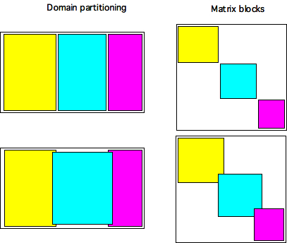\caption{Illustration of block Jacobi and Additive Schwarz preconditioners: left domains and subdomains, right the corresponding submatrices}

Figure  35.1.7.3.3 illustrates these preconditioners both in matrix and subdomain terms.

35.1.7.3.4 Multigrid preconditioners

crumb trail: > petsc-solver > KSP: linear system solvers > Preconditioners > Types > Multigrid preconditioners

• There is a AMG type built into PETSc: PCGAMG ;
• the external packages Hypre and ML have AMG methods.
• There is a general MG type: PCMG  .

35.1.7.3.5 Field split preconditioners

crumb trail: > petsc-solver > KSP: linear system solvers > Preconditioners > Types > Field split preconditioners

For background refer to section  32.4.8  .

Exercise The example code ksp.c generates a five-point matrix, possibly nonsymmetric, on a unit square. Your assignment is to explore the convergence behavior of different solvers on linear systems with this coefficient matrix.

The example code takes two commandline arguments:

• -n 123 set the domain size, meaning that the matrix size will be the square of that;
• -unsymmetry .5 introduces a skew-symmetric component to the matrix.

Investigate the following:

• Some iterative methods, such as CG  , are only mathematically defined for symmetric (and positive definite) matrices. How tolerant are iterative methods actually towards nonsymmetry?
• The number of iterations can sometimes be proved to depend on the condition number of the matrix, which is itself related to the size of the matrix. Can you find a relation between the matrix size and the number of iterations?
• A more sophisticated iterative methods (for instance, increasing the GMRES restart length) or a more sophisticated preconditioner (for instance using more fill levels in an ILU preconditioner), may lead to fewer iterations. (Does it, actually?) But it will not necessarily give a faster solution time, since each iteration is now more expensive.

35.1.7.3.6 Shell preconditioners

crumb trail: > petsc-solver > KSP: linear system solvers > Preconditioners > Types > Shell preconditioners

You already saw that, in an iterative methods, the coefficient matrix can be given operationally as a shell matrix ; section  32.4.7  . Similarly, the preconditioner matrix can be specified operationally by specifying type PCSHELL  .

This needs specification of the application routine through PCShellSetApply :

PCShellSetApply(PC pc,PetscErrorCode (*apply)(PC,Vec,Vec));

PCShellSetContext(PC pc,void *ctx);

PCShellGetContext(PC pc,void **ctx);

If the shell preconditioner requires setup, a routine for this can be specified with PCShellSetSetUp :

PCShellSetSetUp(PC pc,PetscErrorCode (*setup)(PC));

35.1.7.3.7 Combining preconditioners

crumb trail: > petsc-solver > KSP: linear system solvers > Preconditioners > Types > Combining preconditioners

It is possible to combine preconditioners with PCCOMPOSITE

PCSetType(pc,PCCOMPOSITE);
PCCompositeAddPC(pc,type1);
PCCompositeAddPC(pc,type2);

PCCompositeSetType(PC pc,PCCompositeType PC_COMPOSITE_MULTIPLICATIVE);

35.1.8 Customization: monitoring and convergence tests

crumb trail: > petsc-solver > KSP: linear system solvers > Customization: monitoring and convergence tests

PETSc solvers can do various callback s to user functions.

35.1.8.1 Convergence tests

crumb trail: > petsc-solver > KSP: linear system solvers > Customization: monitoring and convergence tests > Convergence tests

For instance, you can set your own convergence test with KSPSetConvergenceTest  .

KSPSetConvergenceTest
   (KSP ksp,
    PetscErrorCode (*test)(
        KSP ksp,PetscInt it,PetscReal rnorm,
        KSPConvergedReason *reason,void *ctx),
    void *ctx,PetscErrorCode (*destroy)(void *ctx));

• the custom stopping test function,
• a `context' void pointer to pass information to the tester, and
• optionally a custom destructor for the context information.

35.1.8.2 Convergence monitoring

crumb trail: > petsc-solver > KSP: linear system solvers > Customization: monitoring and convergence tests > Convergence monitoring

There is also a callback for monitoring each iteration. It can be set with KSPMonitorSet  .

KSPMonitorSet
   (KSP ksp,
    PetscErrorCode (*mon)(
        KSP ksp,PetscInt it,PetscReal rnorm,void *ctx),
    void *ctx,PetscErrorCode (*mondestroy)(void**));

This actually outputs the `preconditioned norm' of the residual, which is not the L2 norm, but the square root of $r^tM\inv r$, a quantity that is computed in the course of the iteration process. Specifying KSPMonitorTrueResidualNorm (with corresponding option ksp_monitor_true_residual  ) as the monitor prints the actual norm $\sqrt{r^tr}$. However, to compute this involves extra computation, since this quantity is not normally computed.

35.1.8.3 Auxiliary routines

crumb trail: > petsc-solver > KSP: linear system solvers > Customization: monitoring and convergence tests > Auxiliary routines

KSPGetSolution KSPGetRhs KSPBuildSolution KSPBuildResidual

KSPGetSolution(KSP ksp,Vec *x);
KSPGetRhs(KSP ksp,Vec *rhs);
KSPBuildSolution(KSP ksp,Vec w,Vec *v);
KSPBuildResidual(KSP ksp,Vec t,Vec w,Vec *v);

35.2 Direct solvers

crumb trail: > petsc-solver > Direct solvers

PETSc has some support for direct solvers, that is, variants of LU decomposition. In a sequential context, the PCLU preconditioner can be use for this: a direct solver is equivalent to an iterative method that stops after one preconditioner application. This can be forced by specifying a KSP type of KSPPREONLY  .

Distributed direct solvers are more complicated. PETSc does not have this implemented in its basic code, but it becomes available by configuring PETSc with the scalapack library.

You need to specify which package provides the LU factorization:

PCFactorSetMatSolverType(pc, MatSolverType solver )

where the solver variable is of type MatSolverType  , and can be MATSOLVERMUMS and such when specified in source:

// direct.c
PetscCall( KSPCreate(comm,&Solver) );
PetscCall( KSPSetOperators(Solver,A,A) );
PetscCall( KSPSetType(Solver,KSPPREONLY) );
{
  PC Prec;
  PetscCall( KSPGetPC(Solver,&Prec) );
  PetscCall( PCSetType(Prec,PCLU) );
  PetscCall( PCFactorSetMatSolverType(Prec,MATSOLVERMUMPS) );
}

yourprog -ksp_type preonly -pc_type lu -pc_factor_mat_solver_type mumps

35.3 Control through command line options

crumb trail: > petsc-solver > Control through command line options

From the above you may get the impression that there are lots of calls to be made to set up a PETSc linear system and solver. And what if you want to experiment with different solvers, does that mean that you have to edit a whole bunch of code? Fortunately, there is an easier way to do things. If you call the routine KSPSetFromOptions with the solver as argument, PETSc will look at your command line options and take those into account in defining the solver. Thus, you can either omit setting options in your source code, or use this as a way of quickly experimenting with different possibilities. Example:

myprogram -ksp_max_it 200 \
    -ksp_type gmres -ksp_type_gmres_restart 20  \
    -pc_type ilu -pc_type_ilu_levels 3