MPI topic: Collectives
Experimental html version of Parallel Programming in MPI, OpenMP, and PETSc by Victor Eijkhout. download the textbook at https:/theartofhpc.com/pcse
3.1.1 : Practical use of collectives
3.1.2 : Synchronization
3.1.3 : Collectives in MPI
3.2 : Reduction
3.2.1 : Reduce to all
3.2.1.1 : Buffer description
3.2.1.2 : Examples and exercises
3.2.2 : Inner product as allreduce
3.2.3 : Reduction operations
3.2.4 : Data buffers
3.3 : Rooted collectives: broadcast, reduce
3.3.1 : Reduce to a root
3.3.2 : Reduce in place
3.3.3 : Broadcast
3.4 : Scan operations
3.4.1 : Exclusive scan
3.4.2 : Use of scan operations
3.5 : Rooted collectives: gather and scatter
3.5.1 : Examples
3.5.2 : Allgather
3.6 : All-to-all
3.6.1 : All-to-all as data transpose
3.6.2 : All-to-all-v
3.7 : Reduce-scatter
3.7.1 : Examples
3.8 : Barrier
3.9 : Variable-size-input collectives
3.9.1 : Example of Gatherv
3.9.2 : Example of Allgatherv
3.9.3 : Variable all-to-all
3.10 : MPI Operators
3.10.1 : Pre-defined operators
3.10.1.1 : Minloc and maxloc
3.10.2 : User-defined operators
3.10.3 : Local reduction
3.11 : Nonblocking collectives
3.11.1 : Examples
3.11.1.1 : Array transpose
3.11.1.2 : Stencils
3.11.2 : Nonblocking barrier
3.12 : Performance of collectives
3.13 : Collectives and synchronization
3.14 : Performance considerations
3.14.1 : Scalability
3.14.2 : Complexity and scalability of collectives
3.14.2.1 : Broadcast
3.15 : Review questions
Back to Table of Contents
3 MPI topic: Collectives
A certain class of MPI routines are called `collective', or more correctly: `collective on a communicator'. This means that if process one in that communicator calls that routine, they all need to call that routine. In this chapter we will discuss collective routines that are about combining the data on all processes in that communicator, but there are also operations such as opening a shared file that are collective, which will be discussed in a later chapter.
3.1 Working with global information
crumb trail: > mpi-collective > Working with global information
If all processes have individual data, for instance the result of a local computation, you may want to bring that information together, for instance to find the maximal computed value or the sum of all values. Conversely, sometimes one processor has information that needs to be shared with all. For this sort of operation, MPI has collectives .
There are various cases, illustrated in figure 3.1 ,
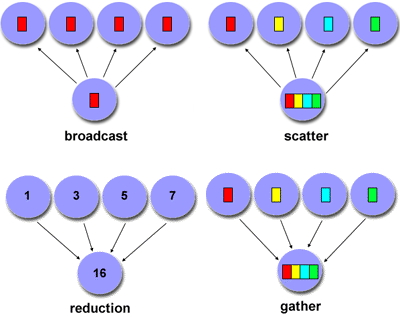
FIGURE 3.1: The four most common collectives
which you can (sort of) motivate by considering some classroom activities:
- The teacher tells the class when the exam will be. This is a broadcast : the same item of information goes to everyone.
- After the exam, the teacher performs a gather operation to collect the invidivual exams.
- On the other hand, when the teacher computes the average grade, each student has an individual number, but these are now combined to compute a single number. This is a reduction .
- Now the teacher has a list of grades and gives each student their grade. This is a scatter operation, where one process has multiple data items, and gives a different one to all the other processes.
This story is a little different from what happens with MPI processes, because these are more symmetric; the process doing the reducing and broadcasting is no different from the others. Any process can function as the root process in such a collective.
Exercise How would you realize the following scenarios with MPI collectives?
- Let each process compute a random number. You want to print the maximum of these numbers to your screen.
- Each process computes a random number again. Now you want to scale these numbers by their maximum.
- Let each process compute a random number. You want to print on what processor the maximum value is computed.
End of exercise
3.1.1 Practical use of collectives
crumb trail: > mpi-collective > Working with global information > Practical use of collectives
Collectives are quite common in scientific applications. For instance, if one process reads data from disc or the commandline, it can use a broadcast or a gather to get the information to other processes. Likewise, at the end of a program run, a gather or reduction can be used to collect summary information about the program run.
However, a more common scenario is that the result of a collective is needed on all processes.
Consider the computation of the standard deviation : \begin{equation} \sigma = \sqrt{\frac1{N-1} \sum_i^N (x_i-\mu)^2 } \qquad\hbox{where}\qquad \mu = \frac{\sum_i^Nx_i}N \end{equation} and assume that every process stores just one $x_i$ value.
- The calculation of the average $\mu$ is a reduction, since all the distributed values need to be added.
- Now every process needs to compute $x_i-\mu$ for its value $x_i$, so $\mu$ is needed everywhere. You can compute this by doing a reduction followed by a broadcast, but it is better to use a so-called allreduce operation, which does the reduction and leaves the result on all processors.
- The calculation of $\sum_i(x_i-\mu)$ is another sum of distributed data, so we need another reduction operation. Depending on whether each process needs to know $\sigma$, we can again use an allreduce.
\begin{equation} y- (x^ty)x \end{equation} Eijkhout:IntroHPC .
3.1.2 Synchronization
crumb trail: > mpi-collective > Working with global information > Synchronization
Collectives are operations that involve all processes in a communicator. %%(See section sec:collectiveslist for an informal listing.) A collective is a single call, and it blocks on all processors, meaning that a process calling a collective cannot proceed until the other processes have similarly called the collective.
That does not mean that all processors exit the call at the same time: because of implementational details and network latency they need not be synchronized in their execution. However, semantically we can say that a process can not finish a collective until every other process has at least started the collective.
In addition to these collective operations, there are operations that are said to be `collective on their communicator', but which do not involve data movement. Collective then means that all processors must call this routine; not to do so is an error that will manifest itself in `hanging' code. One such example is MPI_File_open .
3.1.3 Collectives in MPI
crumb trail: > mpi-collective > Working with global information > Collectives in MPI
We will now explain the MPI collectives in the following order.
- [Allreduce] We use the allreduce as an introduction to the concepts behind collectives; section 3.2 . As explained above, this routines serves many practical scenarios.
- [Broadcast and reduce] We then introduce the concept of a root in the reduce (section 3.3.1 ) and broadcast (section 3.3.3 ) collectives.
- Sometimes you want a reduction with partial results, where each processor computes the sum (or other operation) on the values of lower-numbered processors. For this, you use a scan collective (section 3.4 ).
- [Gather and scatter] The gather/scatter collectives deal with more than a single data item; section 3.5 .
There are more collectives or variants on the above.
- If every processor needs to broadcast to every other, you use an all-to-all operation (section 3.6 ).
- The reduce-scatter is a lesser known combination of collectives; section 3.7 .
- A barrier is an operation that makes all processes wait until every process has reached the barrier (section 3.8 ).
- If you want to gather or scatter information, but the contribution of each processor is of a different size, there are `variable' collectives; they have a v in the name (section 3.9 ).
Finally, there are some advanced topics in collectives.
- User-defined reduction operators; section 3.10.2 .
- Nonblocking collectives; section 3.11 .
- We briefly discuss performance aspects of collectives in section 3.12 .
- We discuss synchronization aspects in section 3.13 .
3.2 Reduction
crumb trail: > mpi-collective > Reduction
3.2.1 Reduce to all
crumb trail: > mpi-collective > Reduction > Reduce to all
Above we saw a couple of scenarios where a quantity is reduced, with all proceses getting the result. The MPI call for this is MPI_Allreduce .
Example: we give each process a random number, and sum these numbers together. The result should be approximately $1/2$ times the number of processes.
// allreduce.c
float myrandom,sumrandom;
myrandom = (float) rand()/(float)RAND_MAX;
// add the random variables together
MPI_Allreduce(&myrandom,&sumrandom,
		1,MPI_FLOAT,MPI_SUM,comm);
// the result should be approx nprocs/2:
if (procno==nprocs-1)
  printf("Result %6.9f compared to .5\n",sumrandom/nprocs);
Or:
MPI_Count buffersize = 1000;
double *indata,*outdata;
indata = (double*) malloc( buffersize*sizeof(double) );
outdata = (double*) malloc( buffersize*sizeof(double) );
MPI_Allreduce_c(indata,outdata,buffersize,MPI_DOUBLE,MPI_SUM,MPI_COMM_WORLD);
3.2.1.1 Buffer description
crumb trail: > mpi-collective > Reduction > Reduce to all > Buffer description
This is the first example in this course that involves MPI data buffers: the MPI_Allreduce call contains two buffer arguments. In most MPI calls (with the one-sided ones as big exception) a buffer is described by three parameters:
- a pointer to the data,
- the number of items in the buffer, and
- the datatype of the items in the buffer.
- The buffer specification depends on the programming languages. Defailts are in section 3.2.4 .
- The count was a 4-byte integer in MPI standard up to and including MPI-3. In the MPI-4 standard the MPI_Count data type become allowed. See section 6.4 for details.
- Datatypes can be predefined, as in the above example, or user-defined. See chapter MPI topic: Data types for details.
Remark
Routines with both a send and receive buffer should not alias these.
Instead, see the discussion of
MPI_IN_PLACE
;
section
3.3.2
.
End of remark
3.2.1.2 Examples and exercises
crumb trail: > mpi-collective > Reduction > Reduce to all > Examples and exercises
Exercise Let each process compute a random number, and compute the sum of these numbers using the MPI_Allreduce routine. \begin{equation} \xi = \sum_i x_i \end{equation}
Each process then scales its value
by this sum.
\begin{equation}
x_i' \leftarrow x_i/ \xi
\end{equation}
Compute the sum of the scaled numbers
\begin{equation}
\xi' = \sum_i x_i'
\end{equation}
and check that it is 1.
(There is a skeleton code randommax in the repository)
End of exercise
Exercise Implement a (very simple-minded) Fourier transform: if $f$ is a function on the interval $[0,1]$, then the $n$-th Fourier coefficient is \begin{equation} f_n\hat = \int_0^1 f(t)e^{-2\pi x}\,dx \end{equation} which we approximate by \begin{equation} f_n\hat = \sum_{i=0}^{N-1} f(ih)e^{-in\pi/N} \end{equation}
- Make one distributed array for the $e^{-inh}$ coefficients,
- make one distributed array for the $f(ih)$ values
- calculate a couple of coefficients
End of exercise
Exercise
In the previous exercise you worked with a distributed array,
computing a local quantity and combining that into a global
quantity.
Why is it not a good idea to gather the whole distributed array on a
single processor, and do all the computation locally?
End of exercise
MPL note The usual reduction operators are given as templated operators:
float
  xrank = static_cast<float>( comm_world.rank() ),
  xreduce;
// separate recv buffer
comm_world.allreduce(mpl::plus<float>(), xrank,xreduce);
// in place
comm_world.allreduce(mpl::plus<float>(), xrank);
The reduction operator has to be compatible with T(T,T)> End of MPL note
For more about operators, see section 3.10 .
3.2.2 Inner product as allreduce
crumb trail: > mpi-collective > Reduction > Inner product as allreduce
One of the more common applications of the reduction operation is the inner product computation. Typically, you have two vectors $x,y$ that have the same distribution, that is, where all processes store equal parts of $x$ and $y$. The computation is then
local_inprod = 0;
for (i=0; i<localsize; i++)
  local_inprod += x[i]*y[i];
MPI_Allreduce( &local_inprod, &global_inprod, 1,MPI_DOUBLE ... )
Exercise The Gram-Schmidt method is a simple way to orthogonalize two vectors: \begin{equation} u \leftarrow u- (u^tv)/(u^tu) \end{equation} Implement this, and check that the result is indeed orthogonal.
Suggestion: fill $v$ with the values $\sin 2nh\pi$ where $n=2\pi/N$,
and $u$ with $\sin 2nh\pi + \sin 4nh\pi$. What does $u$ become after orthogonalization?
End of exercise
3.2.3 Reduction operations
crumb trail: > mpi-collective > Reduction > Reduction operations
Several MPI_Op values are pre-defined. For the list, see section 3.10.1 .
For use in reductions and scans it is possible to define your own operator.
MPI_Op_create( MPI_User_function *func, int commute, MPI_Op *op);
For more details, see section 3.10.2 .
3.2.4 Data buffers
crumb trail: > mpi-collective > Reduction > Data buffers
Collectives are the first example you see of MPI routines that involve transfer of user data. Here, and in every other case, you see that the data description involves:
- A buffer. This can be a scalar or an array.
- A datatype. This describes whether the buffer contains integers, single/double floating point numbers, or more complicated types, to be discussed later.
- A count. This states how many of the elements of the given datatype are in the send buffer, or will be received into the receive buffer.
In the various languages such a buffer/count/datatype triplet is specified in different ways.
First of all, in C the buffer is always an opaque handle , that is, a void* parameter to which you supply an address. This means that an MPI call can take two forms.
For scalars we need to use the ampersand operator to take the address:
float x,y;
MPI_Allreduce( &x,&y,1,MPI_FLOAT, ... );
But for arrays we use the fact that arrays and addresses are more-or-less equivalent in:
float xx[2],yy[2];
MPI_Allreduce( xx,yy,2,MPI_FLOAT, ... );
You could cast the buffers and write:
MPI_Allreduce( (void*)&x,(void*)&y,1,MPI_FLOAT, ... );
MPI_Allreduce( (void*)xx,(void*)yy,2,MPI_FLOAT, ... );
but that is not necessary. The compiler will not complain if you leave out the cast.
C++ note Treatment of scalars in C++ is the same as in C. However, for arrays you have the choice between C-style arrays, and \lstinline+std::vector+ or std::array . For the latter there are two ways of dealing with buffers:
vector<float> xx(25);
MPI_Send( xx.data(),25,MPI_FLOAT, .... );
MPI_Send( &xx[0],25,MPI_FLOAT, .... );
End of C++ note
Fortran note In Fortran parameters are always passed by reference, so the buffer is treated the same way:
Real*4 :: x
Real*4,dimension(2) :: xx
call MPI_Allreduce( x,1,MPI_REAL4, ... )
call MPI_Allreduce( xx,2,MPI_REAL4, ... )
End of Fortran note
In discussing OO languages, we first note that the official C++ API has been removed from the standard.
Specification of the buffer/count/datatype triplet is not needed explicitly in OO languages.
Python note Most MPI routines in Python have both a variant that can send arbitrary Python data, and one that is based on numpy arrays. The former looks the most `pythonic', and is very flexible, but is usually demonstrably inefficient.
## allreduce.py
random_number = random.randint(1,random_bound)
# native mode send
max_random = comm.allreduce(random_number,op=MPI.MAX)
In the numpy variant, all buffers are numpy objects, which carry information about their type and size. For scalar reductions this means we have to create an array for the receive buffer, even though only one element is used.
myrandom = np.empty(1,dtype=int)
myrandom[0] = random_number
allrandom = np.empty(nprocs,dtype=int)
# numpy mode send
comm.Allreduce(myrandom,allrandom[:1],op=MPI.MAX)
Python note In many examples you will pass a whole Numpy array as send/receive buffer. Should want to use a buffer that corresponds to a subset of an array, you can use the following notation:
MPI_Whatever( buffer[...,5] # more stufffor passing the buffer that starts at location 5 of the array.
For even more complicated effects, use numpy.frombuffer : \psnippetwithoutput{pyfrombuf}{examples/mpi/p}{buffer}
MPL note Buffer type handling is done through polymorphism and templating: no explicit indiation of types.
Scalars are handled as such:
float x,y;
comm.bcast( 0,x ); // note: root first
comm.allreduce( mpl::plus<float>(), x,y ); // op first
where the reduction function needs to be compatible with the type of the buffer. End of MPL note
MPL note If your buffer is a std::vector you need to take the .data() component of it:
vector<float> xx(2),yy(2);
comm.allreduce( mpl::plus<float>(),
    xx.data(), yy.data(), mpl::contiguous_layout<float>(2) );
The
contiguous_layout is a `derived type';
this will be discussed in more detail elsewhere
(see note
6.3.1
and later).
For now, interpret it as a way of indicating the count/type
part of a buffer specification.
End of MPL note
MPL note MPL point-to-point routines have a way of specifying the buffer(s) through a begin and end iterator.
// sendrange.cxx
vector<double> v(15);
  comm_world.send(v.begin(), v.end(), 1);  // send to rank 1
  comm_world.recv(v.begin(), v.end(), 0);  // receive from rank 0
3.3 Rooted collectives: broadcast, reduce
crumb trail: > mpi-collective > Rooted collectives: broadcast, reduce
In some scenarios there is a certain process that has a privileged status.
- One process can generate or read in the initial data for a program run. This then needs to be communicated to all other processes.
- At the end of a program run, often one process needs to output some summary information.
3.3.1 Reduce to a root
crumb trail: > mpi-collective > Rooted collectives: broadcast, reduce > Reduce to a root
In the broadcast operation a single data item was communicated to all processes. A reduction operation with MPI_Reduce goes the other way: each process has a data item, and these are all brought together into a single item.
Here are the essential elements of a reduction operation:
MPI_Reduce( senddata, recvdata..., operator,
    root, comm );
- There is the original data, and the data resulting from the reduction. It is a design decision of MPI that it will not by default overwrite the original data. The send data and receive data are of the same size and type: if every processor has one real number, the reduced result is again one real number.
- It is possible to indicate explicitly that a single buffer is used, and thereby the original data overwritten; see section 3.3.2 for this `in place' mode.
- There is a reduction operator. Popular choices are MPI_SUM , MPI_PROD and MPI_MAX , but complicated operators such as finding the location of the maximum value exist. (For the full list, see section 3.10.1 .) You can also define your own operators; section 3.10.2 .
- There is a root process that receives the result of the reduction. Since the nonroot processes do not receive the reduced data, they can actually leave the receive buffer undefined.
// reduce.c
float myrandom = (float) rand()/(float)RAND_MAX,
  result;
int target_proc = nprocs-1;
// add all the random variables together
MPI_Reduce(&myrandom,&result,1,MPI_FLOAT,MPI_SUM,
           target_proc,comm);
// the result should be approx nprocs/2:
if (procno==target_proc)
  printf("Result %6.3f compared to nprocs/2=%5.2f\n",
         result,nprocs/2.);
Exercise Write a program where each process computes a random number, and process 0 finds and prints the maximum generated value. Let each process print its value, just to check the correctness of your program.
(See ch:random for a discussion of random number generation.)
End of exercise
Collective operations can also take an array argument, instead of just a scalar. In that case, the operation is applied pointwise to each location in the array.
Exercise
Create on each process an array of length 2 integers, and put the
values $1,2$ in it on each process. Do a sum reduction on that
array. Can you predict what the result should be? Code it. Was your
prediction right?
End of exercise
3.3.2 Reduce in place
crumb trail: > mpi-collective > Rooted collectives: broadcast, reduce > Reduce in place
By default MPI will not overwrite the original data with the reduction result, but you can tell it to do so using the MPI_IN_PLACE specifier:
// allreduceinplace.c
for (int irand=0; irand<nrandoms; irand++)
	myrandoms[irand] = (float) rand()/(float)RAND_MAX;
// add all the random variables together
MPI_Allreduce(MPI_IN_PLACE,myrandoms,
		    nrandoms,MPI_FLOAT,MPI_SUM,comm);
The above example used MPI_IN_PLACE in MPI_Allreduce ; in MPI_Reduce it's little tricky. The reasoning is a follows:
- In MPI_Reduce every process has a buffer to contribute, but only the root needs a receive buffer. Therefore, MPI_IN_PLACE takes the place of the receive buffer on any processor except for the root \ldots
- … while the root, which needs a receive buffer, has MPI_IN_PLACE takes the place of the send buffer. In order to contribute its value, the root needs to put this in the receive buffer.
Here is one way you could write the in-place version of MPI_Reduce :
if (procno==root)
  MPI_Reduce(MPI_IN_PLACE,myrandoms,
		   nrandoms,MPI_FLOAT,MPI_SUM,root,comm);
else
  MPI_Reduce(myrandoms,MPI_IN_PLACE,
		   nrandoms,MPI_FLOAT,MPI_SUM,root,comm);
float *sendbuf,*recvbuf;
if (procno==root) {
  sendbuf = MPI_IN_PLACE; recvbuf = myrandoms;
} else {
  sendbuf = myrandoms; recvbuf = MPI_IN_PLACE;
}
MPI_Reduce(sendbuf,recvbuf,
  	 nrandoms,MPI_FLOAT,MPI_SUM,root,comm);
In Fortran you can not do these address calculations. You can use the solution with a conditional:
!! reduceinplace.F90
  call random_number(mynumber)
  target_proc = ntids-1;
  ! add all the random variables together
  if (mytid.eq.target_proc) then
     result = mytid
     call MPI_Reduce(MPI_IN_PLACE,result,1,MPI_REAL,MPI_SUM,&
          target_proc,comm)
  else
     mynumber = mytid
     call MPI_Reduce(mynumber,result,1,MPI_REAL,MPI_SUM,&
          target_proc,comm)
  end if
!! reduceinplaceptr.F90
  in_place_val = MPI_IN_PLACE
  if (mytid.eq.target_proc) then
     ! set pointers
     result_ptr => result
     mynumber_ptr => in_place_val
     ! target sets value in receive buffer
     result_ptr = mytid
  else
     ! set pointers
     mynumber_ptr => mynumber
     result_ptr => in_place_val
     ! non-targets set value in send buffer
     mynumber_ptr = mytid
  end if
  call MPI_Reduce(mynumber_ptr,result_ptr,1,MPI_REAL,MPI_SUM,&
       target_proc,comm,err)
Python note The value MPI.IN_PLACE can be used for the send buffer:
## allreduceinplace.py myrandom = np.empty(1,dtype=int) myrandom[0] = random_numbercomm.Allreduce(MPI.IN_PLACE,myrandom,op=MPI.MAX)
MPL note The in-place variant is activated by specifying only one instead of two buffer arguments.
float
  xrank = static_cast<float>( comm_world.rank() ),
  xreduce;
// separate recv buffer
comm_world.allreduce(mpl::plus<float>(), xrank,xreduce);
// in place
comm_world.allreduce(mpl::plus<float>(), xrank);
// collectbuffer.cxx
float
  xrank = static_cast<float>( comm_world.rank() );
vector<float> rank2p2p1{ 2*xrank,2*xrank+1 },reduce2p2p1{0,0};
mpl::contiguous_layout<float> two_floats(rank2p2p1.size());
comm_world.allreduce
  (mpl::plus<float>(), rank2p2p1.data(),reduce2p2p1.data(),two_floats);
if ( iprint )
  cout << "Got: " << reduce2p2p1.at(0) << ","
	 << reduce2p2p1.at(1) << endl;
MPL note End of MPL note MPL note There is a separate variant for non-root usage of rooted collectives:
// scangather.cxx
if (procno==0) {
  comm_world.reduce
    ( mpl::plus<int>(),0,
      my_number_of_elements,total_number_of_elements );
} else {
  comm_world.reduce
    ( mpl::plus<int>(),0,my_number_of_elements );
}
3.3.3 Broadcast
crumb trail: > mpi-collective > Rooted collectives: broadcast, reduce > Broadcast
A broadcast models the scenario where one process, the `root' process, owns some data, and it communicates it to all other processes.
The broadcast routine MPI_Bcast has the following structure:
MPI_Bcast( data..., root , comm);Here:
- There is only one buffer, the send buffer. Before the call, the root process has data in this buffer; the other processes allocate a same sized buffer, but for them the contents are irrelevant.
- The root is the process that is sending its data. Typically, it will be the root of a broadcast tree.
Example: in general we can not assume that all processes get the commandline arguments so we broadcast them from process 0.
// init.c
if (procno==0) {
  if ( argc==1 || // the program is called without parameter
       ( argc>1 && !strcmp(argv[1],"-h") ) // user asked for help
       ) {
    printf("\nUsage: init [0-9]+\n");
    MPI_Abort(comm,1);
  }
  input_argument = atoi(argv[1]);
}
MPI_Bcast(&input_argument,1,MPI_INT,0,comm);
Python note In python it is both possible to send objects, and to send more C-like buffers. The two possibilities correspond (see section 1.5.4 ) to different routine names; the buffers have to be created as numpy objects.
We illustrate both the general Python and numpy variants. In the former variant the result is given as a function return; in the numpy variant the send buffer is reused.
## bcast.py
# first native
if procid==root:
    buffer = [ 5.0 ] * dsize
else:
    buffer = [ 0.0 ] * dsize
buffer = comm.bcast(obj=buffer,root=root)
if not reduce( lambda x,y:x and y,
               [ buffer[i]==5.0 for i in  range(len(buffer)) ] ):
    print( "Something wrong on proc %d: native buffer <<%s>>" \
           % (procid,str(buffer)) )


# then with NumPy
buffer = np.arange(dsize, dtype=np.float64)
if procid==root:
    for i in range(dsize):
        buffer[i] = 5.0
comm.Bcast( buffer,root=root )
if not all( buffer==5.0 ):
    print( "Something wrong on proc %d: numpy buffer <<%s>>" \
           % (procid,str(buffer)) )
else:
    if procid==root:
        print("Success.")
MPL note The broadcast call comes in two variants, with scalar argument and general layout:
 template<typename T >
void mpl::communicator::bcast
   ( int root_rank, T &data ) const;
void mpl::communicator::bcast
   ( int root_rank, T *data, const layout< T > &l ) const;
Note that the root argument comes first. End of MPL note
For the following exercise, study figure fig:gauss-jordan-ex .
Exercise The Gauss-Jordan algorithm for solving a linear system with a matrix $A$ (or computing its inverse) runs as follows:
for pivot $k=1,\ldots,n$
let the vector of scalings $\ell^{(k)}_i=A_{ik}/A_{kk}$
for row $r\not=k$
for column $c=1,\ldots,n$
$A_{rc}\leftarrow A_{rc} - \ell^{(k)}_r A_{kc}$
where we ignore the update of the righthand side, or the formation of the inverse.
Let a matrix be distributed with each process storing one
column. Implement the Gauss-Jordan algorithm as a series of
broadcasts: in iteration $k$ process $k$ computes and broadcasts the
scaling vector $\{\ell^{(k)}_i\}_i$. Replicate the right-hand side on
all processors.
(There is a skeleton code jordan in the repository)
End of exercise
Exercise Add partial pivoting to your implementation of Gauss-Jordan elimination.
Change your implementation to let each processor store multiple columns,
but still do one broadcast per column. Is there a way to have only one
broadcast per processor?
End of exercise
3.4 Scan operations
crumb trail: > mpi-collective > Scan operations
The MPI_Scan operation also performs a reduction, but it keeps the partial results. That is, if processor $i$ contains a number $x_i$, and $\oplus$ is an operator, then the scan operation leaves $x_0\oplus\cdots\oplus x_i$ on processor $i$. This type of operation is often called a prefix operation ; see Eijkhout:IntroHPC .
The MPI_Scan routine is an inclusive scan operation, meaning that it includes the data on the process itself; MPI_Exscan (see section 3.4.1 ) is exclusive, and does not include the data on the calling process.
\begin{equation} \begin{array}{rccccc} \mathrm{process:} &0&1&2&\cdots&p-1\\ \mathrm{data:} &x_0&x_1&x_2&\cdots&x_{p-1}\\ \mathrm{inclusive:}\mathstrut &x_0&x_0\oplus x_1&x_0\oplus x_1\oplus x_2&\cdots&\mathop\oplus_{i=0}^{p-1} x_i\\ \mathrm{exclusive:}\mathstrut &\mathrm{unchanged}&x_0&x_0\oplus x_1&\cdots&\mathop\oplus_{i=0}^{p-2} x_i\\ \end{array} \end{equation}
// scan.c
// add all the random variables together
MPI_Scan(&myrandom,&result,1,MPI_FLOAT,MPI_SUM,comm);
// the result should be approaching nprocs/2:
if (procno==nprocs-1)
  printf("Result %6.3f compared to nprocs/2=%5.2f\n",
         result,nprocs/2.);
In python mode the result is a function return value, with numpy the result is passed as the second parameter.
## scan.py
mycontrib = 10+random.randint(1,nprocs)
myfirst = 0
mypartial = comm.scan(mycontrib)
sbuf = np.empty(1,dtype=int)
rbuf = np.empty(1,dtype=int)
sbuf[0] = mycontrib
comm.Scan(sbuf,rbuf)
You can use any of the given reduction operators, (for the list, see section 3.10.1 ), or a user-defined one. In the latter case, the MPI_Op operations do not return an error code.
MPL note As in the C/F interfaces, MPL interfaces to the scan routines have the same calling sequences as the `Allreduce' routine. End of MPL note
3.4.1 Exclusive scan
crumb trail: > mpi-collective > Scan operations > Exclusive scan
Often, the more useful variant is the exclusive scan MPI_Exscan with the same signature.
The result of the exclusive scan is undefined on processor 0 ( None in python), and on processor 1 it is a copy of the send value of processor 1. In particular, the MPI_Op need not be called on these two processors.
Exercise
The exclusive definition, which computes $x_0\oplus x_{i-1}$ on
processor $i$, can be derived from the inclusive operation
for operations such as
MPI_SUM
or
MPI_PROD
. Are there operators where that is not the
case?
End of exercise
3.4.2 Use of scan operations
crumb trail: > mpi-collective > Scan operations > Use of scan operations
The MPI_Scan operation is often useful with indexing data. Suppose that every processor $p$ has a local vector where the number of elements $n_p$ is dynamically determined. In order to translate the local numbering $0\ldots n_p-1$ to a global numbering one does a scan with the number of local elements as input. The output is then the global number of the first local variable.
As an example, setting FFT coefficients requires this translation. If the local sizes are all equal, determining the global index of the first element is an easy calculation. For the irregular case, we first do a scan:
// fft.c MPI_Allreduce( &localsize,&globalsize,1,MPI_INT,MPI_SUM, comm ); globalsize += 1; int myfirst=0; MPI_Exscan( &localsize,&myfirst,1,MPI_INT,MPI_SUM, comm );for (int i=0; i<localsize; i++) vector[i] = sin( pi*freq* (i+1+myfirst) / globalsize );
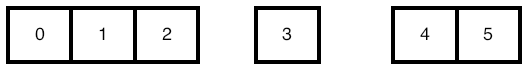
FIGURE 3.2: Local arrays that together form a consecutive range
Exercise
- Let each process compute a random value $n_{\scriptstyle\mathrm{local}}$, and allocate an array of that length. Define \begin{equation} N=\sum n_{\scriptstyle\mathrm{local}} \end{equation}
- Fill the array with consecutive integers, so that all local arrays, laid end-to-end, contain the numbers $0\cdots N-1$. (See figure 3.2 .)
End of exercise
Exercise
Did you use
MPI_Scan
or
MPI_Exscan
for
the previous exercise?
How would you describe the result of the other scan operation, given the
same input?
End of exercise
It is possible to do a segmented scan . Let $x_i$ be a series of numbers that we want to sum to $X_i$ as follows. Let $y_i$ be a series of booleans such that \begin{equation} \begin{cases} X_i=x_i&\hbox{if $y_i=0$}\\ X_i=X_{i-1}+x_i&\hbox{if $y_i=1$} \end{cases} \end{equation} (This is the basis for the implementation of the sparse matrix vector product as prefix operation; see Eijkhout:IntroHPC .) This means that $X_i$ sums the segments between locations where $y_i=0$ and the first subsequent place where $y_i=1$. To implement this, you need a user-defined operator \begin{equation} \begin{pmatrix} X\\ x\\ y \end{pmatrix} = \begin{pmatrix} X_1\\ x_1\\ y_1 \end{pmatrix} \bigoplus \begin{pmatrix} X_2\\ x_2\\ y_2 \end{pmatrix} \colon \begin{cases} X=x_1+x_2&\hbox{if $y_2==1$}\\ X=x_2&\hbox{if $y_2==0$} \end{cases} \end{equation} This operator is not communitative, and it needs to be declared as such with MPI_Op_create ; see section 3.10.2
3.5 Rooted collectives: gather and scatter
crumb trail: > mpi-collective > Rooted collectives: gather and scatter
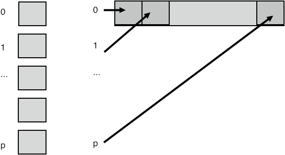
FIGURE 3.3: Gather collects all data onto a root
In the MPI_Scatter operation, the root spreads information to all other processes. The difference with a broadcast is that it involves individual information from/to every process. Thus, the gather operation typically has an array of items, one coming from each sending process, and scatter has an array,
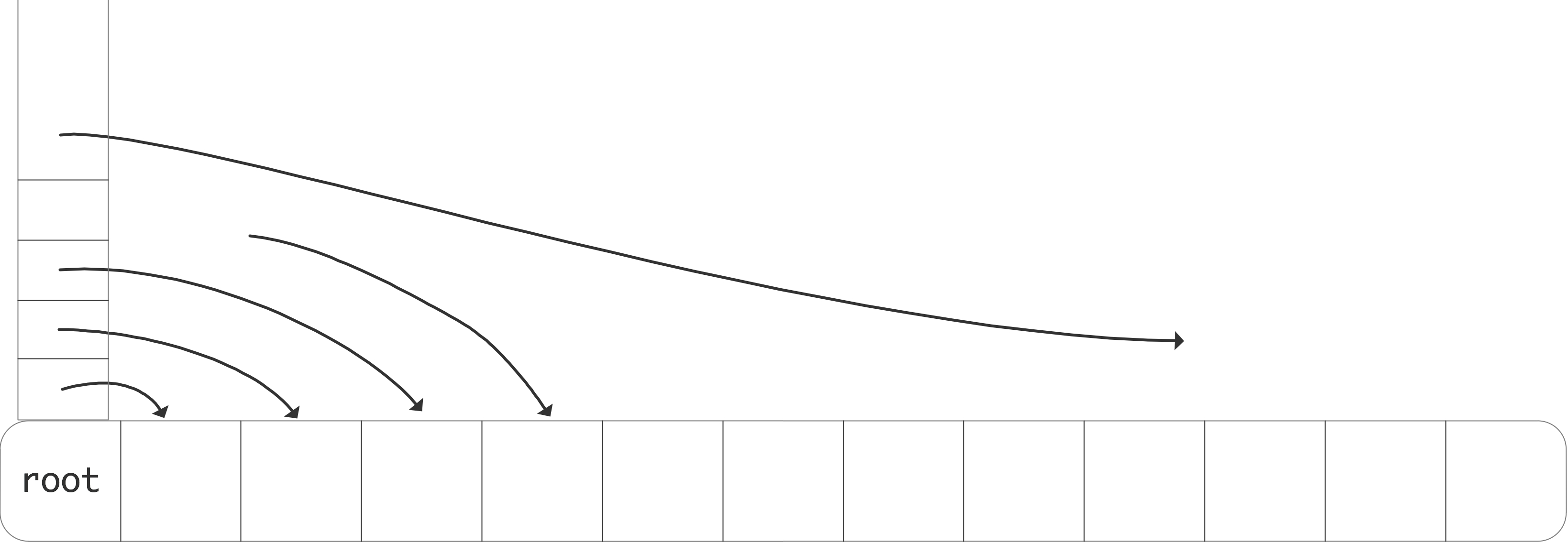
FIGURE 3.4: A scatter operation
with an individual item for each receiving process; see figure 3.4 .
These gather and scatter collectives have a different parameter list from the broadcast/reduce. The broadcast/reduce involves the same amount of data on each process, so it was enough to have a single datatype/size specification; for one buffer in the broadcast, and for both buffers in the reduce call. In the gather/scatter calls you have
- a large buffer on the root, with a datatype and size specification, and
- a smaller buffer on each process, with its own type and size specification.
In the gather and scatter calls, each processor has $n$ elements of individual data. There is also a root processor that has an array of length $np$, where $p$ is the number of processors. The gather call collects all this data from the processors to the root; the scatter call assumes that the information is initially on the root and it is spread to the individual processors.
Here is a small example:
// gather.c // we assume that each process has a value "localsize" // the root process collects these valuesif (procno==root) localsizes = (int*) malloc( nprocs*sizeof(int) );
// everyone contributes their info MPI_Gather(&localsize,1,MPI_INT, localsizes,1,MPI_INT,root,comm);
Exercise
Let each process compute a random number.
You want to print the maximum value and on what processor it
is computed. What collective(s) do you use? Write a short program.
End of exercise
The MPI_Scatter operation is in some sense the inverse of the gather: the root process has an array of length $np$ where $p$ is the number of processors and $n$ the number of elements each processor will receive.
int MPI_Scatter
  (void* sendbuf, int sendcount, MPI_Datatype sendtype,
   void* recvbuf, int recvcount, MPI_Datatype recvtype,
   int root, MPI_Comm comm)
Two things to note about these routines:
- The signature for MPI_Gather has two `count' parameters, one for the length of the individual send buffers, and one for the receive buffer. However, confusingly, the second parameter (which is only relevant on the root) does not indicate the total amount of information coming in, but rather the size of each contribution. Thus, the two count parameters will usually be the same (at least on the root); they can differ if you use different MPI_Datatype values for the sending and receiving processors.
- While every process has a sendbuffer in the gather, and a receive buffer in the scatter call, only the root process needs the long array in which to gather, or from which to scatter. However, because in SPMD mode all processes need to use the same routine, a parameter for this long array is always present. Nonroot processes can use a null pointer here.
- More elegantly, the MPI_IN_PLACE option can be used for buffers that are not applicable, such as the receive buffer on a sending process. See section 3.3.2 .
MPL note Gathering (by communicator:: gather) or scattering (by communicator:: scatter) a single scalar takes a scalar argument and a raw array:
vector<float> v;
float x;
comm_world.scatter(0, v.data(), x);
vector<float> vrecv(2),vsend(2*nprocs);
mpl::contiguous_layout<float> twonums(2);
comm_world.scatter
  (0, vsend.data(),twonums, vrecv.data(),twonums );
MPL note Logically speaking, on every nonroot process, the gather call only has a send buffer. MPL supports this by having two variants that only specify the send data.
if (procno==0) {
  vector<int> size_buffer(nprocs);
  comm_world.gather
    (
     0,my_number_of_elements,size_buffer.data()
     );
} else {
  /*
   * If you are not the root, do versions with only send buffers
   */
  comm_world.gather
    ( 0,my_number_of_elements );
3.5.1 Examples
crumb trail: > mpi-collective > Rooted collectives: gather and scatter > Examples
In some applications, each process computes a row or column of a matrix, but for some calculation (such as the determinant) it is more efficient to have the whole matrix on one process. You should of course only do this if this matrix is essentially smaller than the full problem, such as an interface system or the last coarsening level in multigrid.
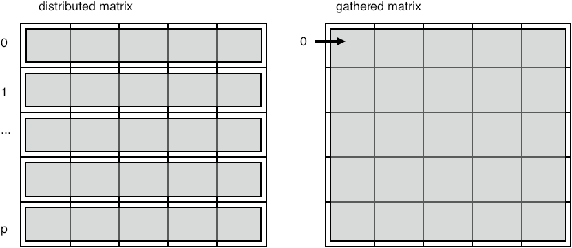
FIGURE 3.5: Gather a distributed matrix onto one process
Figure 3.5 pictures this. Note that conceptually we are gathering a two-dimensional object, but the buffer is of course one-dimensional. You will later see how this can be done more elegantly with the `subarray' datatype; section 6.3.4 .
Another thing you can do with a distributed matrix is to transpose it.
// itransposeblock.c
for (int iproc=0; iproc<nprocs; iproc++) {
  MPI_Scatter( regular,1,MPI_DOUBLE,
		 &(transpose[iproc]),1,MPI_DOUBLE,
		 iproc,comm);
}
Exercise
Can you rewrite this code so that it uses a gather rather than a scatter?
Does that change anything essential about structure of the code?
End of exercise
Exercise Take the code from exercise 3.2 and extend it to gather all local buffers onto rank zero. Since the local arrays are of differing lengths, this requires MPI_Gatherv .
How do you construct the lengths and displacements arrays?
(There is a skeleton code scangather in the repository)
End of exercise
3.5.2 Allgather
crumb trail: > mpi-collective > Rooted collectives: gather and scatter > Allgather
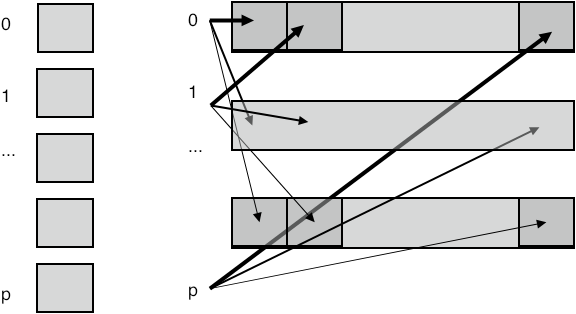
FIGURE 3.6: All gather collects all data onto every process
The MPI_Allgather routine does the same gather onto every process: each process winds up with the totality of all data; figure 3.6 .
This routine can be used in the simplest implementation of the dense matrix-vector product to give each processor the full input; see Eijkhout:IntroHPC .
The MPI_IN_PLACE keyword can be used with an all-gather:
- Use MPI_IN_PLACE for the send buffer;
- send count and datetype are ignored by MPI;
- each process needs to put its `send content' in the correct location of the gather buffer.
Some cases look like an all-gather but can be implemented more efficiently. Let's consider as an example the set difference of two distributed vectors. That is, you have two distributed vectors, and you want to create a new vector, again distributed, that contains those elements of the one that do not appear in the other. You could implement this by gathering the second vector on each processor, but this may be prohibitive in memory usage.
Exercise
Can you think of another algorithm for taking the set difference of
two distributed vectors. Hint: look up
bucket brigade
algorithm;
section
4.1.5
.
What is the time and space complexity
of this algorithm? Can you think of other advantages beside a
reduction in workspace?
End of exercise
3.6 All-to-all
crumb trail: > mpi-collective > All-to-all
The all-to-all operation MPI_Alltoall can be seen as a collection of simultaneous broadcasts or simultaneous gathers. The parameter specification is much like an allgather, with a separate send and receive buffer, and no root specified. As with the gather call, the receive count corresponds to an individual receive, not the total amount.
Unlike the gather call, the send buffer now obeys the same principle: with a send count of 1, the buffer has a length of the number of processes.
3.6.1 All-to-all as data transpose
crumb trail: > mpi-collective > All-to-all > All-to-all as data transpose
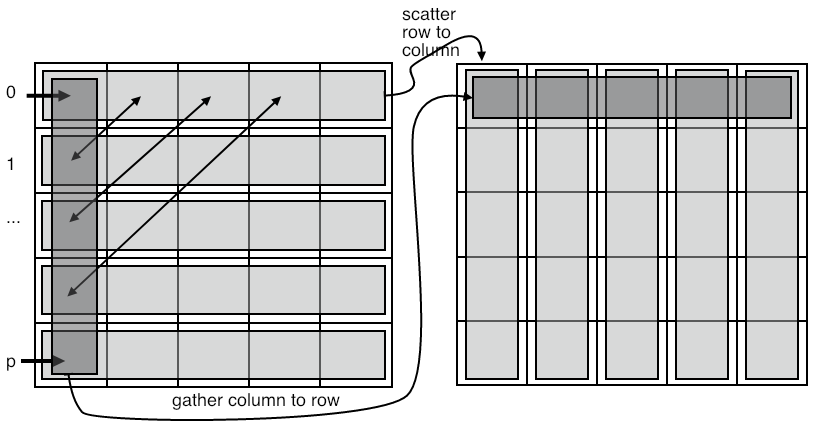
FIGURE 3.7: All-to-all transposes data
The all-to-all operation can be considered as a data transpose. For instance, assume that each process knows how much data to send to every other process. If you draw a connectivity matrix of size $P\times P$, denoting who-sends-to-who, then the send information can be put in rows: \begin{equation} \forall_i\colon C[i,j]>0\quad\hbox{if process $i$ sends to process $j$}. \end{equation} Conversely, the columns then denote the receive information: \begin{equation} \forall_j\colon C[i,j]>0\quad\hbox{if process $j$ receives from process $i$}. \end{equation}
The typical application for such data transposition is in the FFT algorithm, where it can take tens of percents of the running time on large clusters.
We will consider another application of data transposition, namely radix sort , but we will do that in a couple of steps. First of all:
Exercise
In the initial stage of a
radix sort
, each process
considers how many elements to send to every other process.
Use
MPI_Alltoall
to derive from this how many
elements they will receive from every other process.
End of exercise
3.6.2 All-to-all-v
crumb trail: > mpi-collective > All-to-all > All-to-all-v
The major part of the radix sort algorithm consist of every process sending some of its elements to each of the other processes. The routine MPI_Alltoallv is used for this pattern:
- Every process scatters its data to all others,
- but the amount of data is different per process.
Exercise
The actual data shuffle of a
radix sort
can be done
with
MPI_Alltoallv
. Finish the code of
exercise
3.7
.
End of exercise
3.7 Reduce-scatter
crumb trail: > mpi-collective > Reduce-scatter
There are several MPI collectives that are functionally equivalent to a combination of others. You have already seen MPI_Allreduce which is equivalent to a reduction followed by a broadcast. Often such combinations can be more efficient than using the individual calls; see Eijkhout:IntroHPC .
Here is another example: MPI_Reduce_scatter is equivalent to a reduction on an array of data (meaning a pointwise reduction on each array location) followed by a scatter of this array to the individual processes.
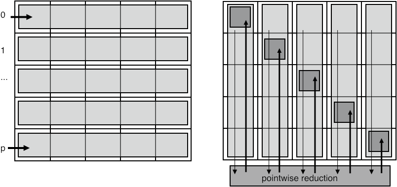
FIGURE 3.8: Reduce scatter
We will discuss this routine, or rather its variant MPI_Reduce_scatter_block , using an important example: the sparse matrix-vector product (see Eijkhout:IntroHPC for background information). Each process contains one or more matrix rows, so by looking at indices the process can decide what other processes it needs to receive data from, that is, each process knows how many messages it will receive, and from which processes. The problem is for a process to find out what other processes it needs to send data to.
Let's set up the data:
// reducescatter.c
int
// data that we know:
  *i_recv_from_proc = (int*) malloc(nprocs*sizeof(int)),
  *procs_to_recv_from, nprocs_to_recv_from=0,
// data we are going to determin:
  *procs_to_send_to,nprocs_to_send_to;
Each process creates an array of ones and zeros, describing who it needs data from. Ideally, we only need the array procs_to_recv_from but initially we need the (possibly much larger) array i_recv_from_proc .
Next, the MPI_Reduce_scatter_block call then computes, on each process, how many messages it needs to send.
MPI_Reduce_scatter_block
  (i_recv_from_proc,&nprocs_to_send_to,1,MPI_INT,
  MPI_SUM,comm);
We do not yet have the information to which processes to send. For that, each process sends a zero-size message to each of its senders. Conversely, it then does a receive to with MPI_ANY_SOURCE to discover who is requesting data from it. The crucial point to the MPI_Reduce_scatter_block call is that, without it, a process would not know how many of these zero-size messages to expect.
/*
 * Send a zero-size msg to everyone that you receive from,
 * just to let them know that they need to send to you.
 */
MPI_Request send_requests[nprocs_to_recv_from];
for (int iproc=0; iproc<nprocs_to_recv_from; iproc++) {
  int proc=procs_to_recv_from[iproc];
  double send_buffer=0.;
  MPI_Isend(&send_buffer,0,MPI_DOUBLE, /*to:*/ proc,0,comm,
	      &(send_requests[iproc]));
}


/*
 * Do as many receives as you know are coming in;
 * use wildcards since you don't know where they are coming from.
 * The source is a process you need to send to.
 */
procs_to_send_to = (int*)malloc( nprocs_to_send_to * sizeof(int) );
for (int iproc=0; iproc<nprocs_to_send_to; iproc++) {
  double recv_buffer;
  MPI_Status status;
  MPI_Recv(&recv_buffer,0,MPI_DOUBLE,MPI_ANY_SOURCE,MPI_ANY_TAG,comm,
	     &status);
  procs_to_send_to[iproc] = status.MPI_SOURCE;
}
MPI_Waitall(nprocs_to_recv_from,send_requests,MPI_STATUSES_IGNORE);
The MPI_Reduce_scatter call is more general: instead of indicating the mere presence of a message between two processes, by having individual receive counts one can, for instance, indicate the size of the messages.
We can look at reduce-scatter as a limited form of the all-to-all data transposition discussed above (section 3.6.1 ). Suppose that the matrix $C$ contains only $0/1$, indicating whether or not a messages is send, rather than the actual amounts. If a receiving process only needs to know how many messages to receive, rather than where they come from, it is enough to know the column sum, rather than the full column (see figure 3.8 ).
Another application of the reduce-scatter mechanism is in the dense matrix-vector product, if a two-dimensional data distribution is used.
Exercise Implement the dense matrix-vector product, where the matrix is distributed by columns: each process stores $A_{*j}$ for a disjoint set of $j$-values. At the start and end of the algorithm each process should store a distinct part of the input and output vectors. Argue that this can be done naively with an MPI_Reduce operation, but more efficiently using MPI_Reduce_scatter .
For discussion, see
Eijkhout:IntroHPC
.
End of exercise
3.7.1 Examples
crumb trail: > mpi-collective > Reduce-scatter > Examples
An important application of this is establishing an irregular communication pattern. Assume that each process knows which other processes it wants to communicate with; the problem is to let the other processes know about this. The solution is to use MPI_Reduce_scatter to find out how many processes want to communicate with you
MPI_Reduce_scatter_block
  (i_recv_from_proc,&nprocs_to_send_to,1,MPI_INT,
  MPI_SUM,comm);
/*
 * Send a zero-size msg to everyone that you receive from,
 * just to let them know that they need to send to you.
 */
MPI_Request send_requests[nprocs_to_recv_from];
for (int iproc=0; iproc<nprocs_to_recv_from; iproc++) {
  int proc=procs_to_recv_from[iproc];
  double send_buffer=0.;
  MPI_Isend(&send_buffer,0,MPI_DOUBLE, /*to:*/ proc,0,comm,
	      &(send_requests[iproc]));
}


/*
 * Do as many receives as you know are coming in;
 * use wildcards since you don't know where they are coming from.
 * The source is a process you need to send to.
 */
procs_to_send_to = (int*)malloc( nprocs_to_send_to * sizeof(int) );
for (int iproc=0; iproc<nprocs_to_send_to; iproc++) {
  double recv_buffer;
  MPI_Status status;
  MPI_Recv(&recv_buffer,0,MPI_DOUBLE,MPI_ANY_SOURCE,MPI_ANY_TAG,comm,
	     &status);
  procs_to_send_to[iproc] = status.MPI_SOURCE;
}
MPI_Waitall(nprocs_to_recv_from,send_requests,MPI_STATUSES_IGNORE);
Use of MPI_Reduce_scatter to implement the two-dimensional matrix-vector product. Set up separate row and column communicators with MPI_Comm_split , use MPI_Reduce_scatter to combine local products.
MPI_Allgather(&my_x,1,MPI_DOUBLE,
   	  local_x,1,MPI_DOUBLE,environ.col_comm);
MPI_Reduce_scatter(local_y,&my_y,&ione,MPI_DOUBLE,
	  MPI_SUM,environ.row_comm);
3.8 Barrier
crumb trail: > mpi-collective > Barrier
A barrier call, MPI_Barrier is a routine that blocks all processes until they have all reached the barrier call. Thus it achieves time synchronization of the processes.
This call's simplicity is contrasted with its usefulness, which is very limited. It is almost never necessary to synchronize processes through a barrier: for most purposes it does not matter if processors are out of sync. Conversely, collectives (except the new nonblocking ones; section 3.11 ) introduce a barrier of sorts themselves.
3.9 Variable-size-input collectives
crumb trail: > mpi-collective > Variable-size-input collectives
In the gather and scatter call above each processor received or sent an identical number of items. In many cases this is appropriate, but sometimes each processor wants or contributes an individual number of items.
Let's take the gather calls as an example. Assume that each processor does a local computation that produces a number of data elements, and this number is different for each processor (or at least not the same for all). In the regular MPI_Gather call the root processor had a buffer of size $nP$, where $n$ is the number of elements produced on each processor, and $P$ the number of processors. The contribution from processor $p$ would go into locations $pn,\ldots,(p+1)n-1$.
For the variable case, we first need to compute the total required buffer size. This can be done through a simple MPI_Reduce with MPI_SUM as reduction operator: the buffer size is $\sum_p n_p$ where $n_p$ is the number of elements on processor $p$. But you can also postpone this calculation for a minute.
The next question is where the contributions of the processor will
go into this buffer. For the contribution from processor $p$
that is $\sum_{q
We now have all the ingredients. All the processors specify a send buffer just as with MPI_Gather . However, the receive buffer specification on the root is more complicated. It now consists of:
outbuffer, array-of-outcounts, array-of-displacements, outtypeand you have just seen how to construct that information.
For example, in an MPI_Gatherv call each process has an individual number of items to contribute. To gather this, the root process needs to find these individual amounts with an MPI_Gather call, and locally construct the offsets array. Note how the offsets array has size ntids+1 : the final offset value is automatically the total size of all incoming data. See the example below.
There are various calls where processors can have buffers of differing sizes.
- In MPI_Scatterv the root process has a different amount of data for each recipient.
- In MPI_Gatherv , conversely, each process contributes a different sized send buffer to the received result; MPI_Allgatherv does the same, but leaves its result on all processes; MPI_Alltoallv does a different variable-sized gather on each process.
3.9.1 Example of Gatherv
crumb trail: > mpi-collective > Variable-size-input collectives > Example of Gatherv
We use MPI_Gatherv to do an irregular gather onto a root. We first need an MPI_Gather to determine offsets. \csnippetwithoutput{gatherv}{examples/mpi/c}{gatherv}
## gatherv.py
# implicitly using root=0
globalsize = comm.reduce(localsize)
if procid==0:
    print("Global size=%d" % globalsize)
collecteddata = np.empty(globalsize,dtype=int)
counts = comm.gather(localsize)
comm.Gatherv(localdata, [collecteddata, counts])
MPL note layouts object, layouts,
End of MPL note
3.9.2 Example of Allgatherv
crumb trail: > mpi-collective > Variable-size-input collectives > Example of Allgatherv
Prior to the actual gatherv call, we need to construct the count and displacement arrays. The easiest way is to use a reduction.
// allgatherv.c
MPI_Allgather
  ( &my_count,1,MPI_INT,
    recv_counts,1,MPI_INT, comm );
int accumulate = 0;
for (int i=0; i<nprocs; i++) {
  recv_displs[i] = accumulate; accumulate += recv_counts[i]; }
int *global_array = (int*) malloc(accumulate*sizeof(int));
MPI_Allgatherv
  ( my_array,procno+1,MPI_INT,
    global_array,recv_counts,recv_displs,MPI_INT, comm );
In python the receive buffer has to contain the counts and displacements arrays.
## allgatherv.py
mycount = procid+1
my_array = np.empty(mycount,dtype=np.float64)
my_count = np.empty(1,dtype=int) my_count[0] = mycount comm.Allgather( my_count,recv_counts )accumulate = 0 for p in range(nprocs): recv_displs[p] = accumulate; accumulate += recv_counts[p] global_array = np.empty(accumulate,dtype=np.float64) comm.Allgatherv( my_array, [global_array,recv_counts,recv_displs,MPI.DOUBLE] )
3.9.3 Variable all-to-all
crumb trail: > mpi-collective > Variable-size-input collectives > Variable all-to-all
The variable all-to-all routine MPI_Alltoallv is discussed in section 3.6.2 .
3.10 MPI Operators
crumb trail: > mpi-collective > MPI Operators
MPI operators , that is, objects of type MPI_Op , are used in reduction operators. Most common operators, such as sum or maximum, have been built into the MPI library; see section 3.10.1 . It is also possible to define new operators; see section 3.10.2 .
3.10.1 Pre-defined operators
crumb trail: > mpi-collective > MPI Operators > Pre-defined operators
The following is the list of pre-defined operators MPI_Op values.
| \toprule MPI type | meaning | applies to |
| \midrule MPI_MAX | maximum | integer, floating point |
| MPI_MIN | minimum | |
| MPI_SUM | sum | integer, floating point, complex, multilanguage types |
| MPI_REPLACE | overwrite | |
| MPI_NO_OP | no change | |
| MPI_PROD | product | |
| MPI_LAND | logical and | C integer, logical |
| MPI_LOR | logical or | |
| MPI_LXOR | logical xor | |
| MPI_BAND | bitwise and | integer, byte, multilanguage types |
| MPI_BOR | bitwise or | |
| MPI_BXOR | bitwise xor | |
| MPI_MAXLOC | max value and location | MPI_DOUBLE_INT and such |
| MPI_MINLOC | min value and location | |
| \bottomrule |
3.10.1.1 Minloc and maxloc
crumb trail: > mpi-collective > MPI Operators > Pre-defined operators > Minloc and maxloc
The MPI_MAXLOC and MPI_MINLOC operations yield both the maximum and the rank on which it occurs. Their result is a struct of the data over which the reduction happens, and an int.
In C, the types to use in the reduction call are: MPI_FLOAT_INT , MPI_LONG_INT , MPI_DOUBLE_INT , MPI_SHORT_INT , MPI_2INT , MPI_LONG_DOUBLE_INT . Likewise, the input needs to consist of such structures: the input should be an array of such struct types, where the int is the rank of the number.
These types may have some unusual size properties: \csnippetwithoutput{longintsize}{examples/mpi/c}{longint}
Fortran note The original Fortran interface to MPI was designed around Fortran77 features, so it is not using Fortran derived types ( Type keyword). Instead, all integer indices are stored in whatever the type is that is being reduced. The available result types are then MPI_2REAL , MPI_2DOUBLE_PRECISION , MPI_2INTEGER .
Likewise, the input needs to be arrays of such type. Consider this example:
Real*8,dimension(2,N) :: input,output
call MPI_Reduce( input,output, N, MPI_2DOUBLE_PRECISION, &
    MPI_MAXLOC, root, comm )
End of Fortran note
MPL note Arithmetic: plus, multiplies, max, min.
Logic: logical_and, logical_or, logical_xor.
Bitwise: bit_and, bit_or, bit_xor. End of MPL note
3.10.2 User-defined operators
crumb trail: > mpi-collective > MPI Operators > User-defined operators
In addition to predefined operators, MPI has the possibility of user-defined operators to use in a reduction or scan operation.
The routine for this is MPI_Op_create , which takes a user function and turns it into an object of type MPI_Op , which can then be used in any reduction:
MPI_Op rwz;
MPI_Op_create(reduce_without_zero,1,&rwz);
MPI_Allreduce(data+procno,&positive_minimum,1,MPI_INT,rwz,comm);
Python note In python, \lstinline+Op.Create+ is a class method for the MPI class.
rwz = MPI.Op.Create(reduceWithoutZero)
positive_minimum = np.zeros(1,dtype=intc)
comm.Allreduce(data[procid],positive_minimum,rwz);
The user function needs to have the following signature:
typedef void MPI_User_function
    ( void *invec, void *inoutvec, int *len,
      MPI_Datatype *datatype);
FUNCTION USER_FUNCTION( INVEC(*), INOUTVEC(*), LEN, TYPE)
<type> INVEC(LEN), INOUTVEC(LEN)
INTEGER LEN, TYPE
For example, here is an operator for finding the smallest nonzero number in an array of nonnegative integers:
*(int*)inout = m;
}
Python note The python equivalent of such a function receives bare buffers as arguments. Therefore, it is best to turn them first into NumPy arrays using np.frombuffer :
## reductpositive.py
def reduceWithoutZero(in_buf, inout_buf, datatype):
    typecode = MPI._typecode(datatype)
    assert typecode is not None ## check MPI datatype is built-in
    dtype = np.dtype(typecode)


    in_array = np.frombuffer(in_buf, dtype)
    inout_array = np.frombuffer(inout_buf, dtype)


    n = in_array[0]; r = inout_array[0]
    if n==0:
        m = r
    elif r==0:
        m = n
    elif n<r:
        m = n
    else:
        m = r
    inout_array[0] = m
MPL note A user-defined operator can be a templated class with an operator() . Example:
// reduceuser.cxx
template<typename T>
class lcm {
public:
  T operator()(T a, T b) {
    T zero=T();
    T t((a/gcd(a, b))*b);
    if (t<zero)
      return -t;
    return t;
  }
comm_world.reduce(lcm<int>(), 0, v, result);
MPL note You can also do the reduction by lambda:
comm_world.reduce
  ( [] (int i,int j) -> int
       { return i+j; },
	0,data );
The function has an array length argument len , to allow for pointwise reduction on a whole array at once. The inoutvec array contains partially reduced results, and is typically overwritten by the function.
There are some restrictions on the user function:
- It may not call MPI functions, except for MPI_Abort .
- It must be associative; it can be optionally commutative, which fact is passed to the MPI_Op_create call.
Exercise
Write the reduction function to implement the
one-norm
of a vector:
\begin{equation}
\|x\|_1 \equiv \sum_i |x_i|.
\end{equation}
(There is a skeleton code onenorm in the repository)
End of exercise
The operator can be destroyed with a corresponding MPI_Op_free .
int MPI_Op_free(MPI_Op *op)This sets the operator to MPI_OP_NULL . This is not necessary in OO languages, where the destructor takes care of it.
You can query the commutativity of an operator with MPI_Op_commutative .
3.10.3 Local reduction
crumb trail: > mpi-collective > MPI Operators > Local reduction
The application of an MPI_Op can be performed with the routine MPI_Reduce_local . Using this routine and some send/receive scheme you can build your own global reductions. Note that this routine does not take a communicator because it is purely local.
3.11 Nonblocking collectives
crumb trail: > mpi-collective > Nonblocking collectives
Above you have seen how the `Isend' and `Irecv' routines can overlap communication with computation. This is not possible with the collectives you have seen so far: they act like blocking sends or receives. However, there are also nonblocking collectives , introduced in MPI-3.
Such operations can be used to increase efficiency. For instance, computing \begin{equation} y \leftarrow Ax + (x^tx)y \end{equation} involves a matrix-vector product, which is dominated by computation in the sparse matrix case, and an inner product which is typically dominated by the communication cost. You would code this as
MPI_Iallreduce( .... x ..., &request);
// compute the matrix vector product
MPI_Wait(request);
// do the addition
This can also be used for 3D FFT operations [Hoefler:case-for-nbc] . Occasionally, a nonblocking collective can be used for nonobvious purposes, such as the MPI_Ibarrier in [Hoefler:2010:SCP] .
These have roughly the same calling sequence as their blocking counterparts, except that they output an MPI_Request . You can then use an MPI_Wait call to make sure the collective has completed.
Nonblocking collectives offer a number of performance advantages:
-
Do two reductions (on the same communicator) with different
operators simultaneously:
\begin{equation}
\begin{array}{l}
\alpha\leftarrow x^ty\\
\beta\leftarrow \|z\|_\infty
\end{array}
\end{equation}
which translates to:
MPI_Allreduce( &local_xy,  &global_xy, 1,MPI_DOUBLE,MPI_SUM,comm);
MPI_Allreduce( &local_xinf,&global_xin,1,MPI_DOUBLE,MPI_MAX,comm);
- do collectives on overlapping communicators simultaneously;
- overlap a nonblocking collective with a blocking one.
Exercise
Revisit exercise
7.1
. Let only the first row and
first column have certain data, which they broadcast through columns
and rows respectively. Each process is now involved in two
simultaneous collectives. Implement this with nonblocking
broadcasts, and time the difference between a blocking and a
nonblocking solution.
(There is a skeleton code procgridnonblock in the repository)
End of exercise
Remark Blocking and nonblocking don't match: either all processes call the nonblocking or all call the blocking one. Thus the following code is incorrect:
if (rank==root)
  MPI_Reduce( &x /* ... */ root,comm );
else
  MPI_Ireduce( &x /* ... */ );
This is unlike the point-to-point behavior of nonblocking calls: you can catch a message with MPI_Irecv that was sent with MPI_Send .
End of remark
Remark
Unlike sends and received, collectives have no identifying tag.
With blocking collectives that does not lead to ambiguity problems.
With nonblocking collectives it means that all processes
need to issue them in identical order.
End of remark
List of nonblocking collectives:
- MPI_Igather , MPI_Igatherv , MPI_Iallgather , MPI_Iallgatherv ,
- MPI_Iscatter , MPI_Iscatterv ,
- MPI_Ireduce , MPI_Iallreduce , MPI_Ireduce_scatter , MPI_Ireduce_scatter_block .
- MPI_Ialltoall , MPI_Ialltoallv , MPI_Ialltoallw ,
- MPI_Ibarrier ; section 3.11.2 ,
- MPI_Ibcast ,
- MPI_Iexscan , MPI_Iscan ,
MPL note Nonblocking collectives have the same argument list as the corresponding blocking variant, except that instead of a void result, they return an irequest. (See 4.2.2 )
// ireducescalar.cxx
float x{1.},sum;
auto reduce_request =
  comm_world.ireduce(mpl::plus<float>(), 0, x, sum);
reduce_request.wait();
if (comm_world.rank()==0) {
  std::cout << "sum = " << sum << '\n';
}
3.11.1 Examples
crumb trail: > mpi-collective > Nonblocking collectives > Examples
3.11.1.1 Array transpose
crumb trail: > mpi-collective > Nonblocking collectives > Examples > Array transpose
To illustrate the overlapping of multiple nonblocking collectives, consider transposing a data matrix. Initially, each process has one row of the matrix; after transposition each process has a column. Since each row needs to be distributed to all processes, algorithmically this corresponds to a series of scatter calls, one originating from each process.
// itransposeblock.c
for (int iproc=0; iproc<nprocs; iproc++) {
  MPI_Scatter( regular,1,MPI_DOUBLE,
		 &(transpose[iproc]),1,MPI_DOUBLE,
		 iproc,comm);
}
MPI_Request scatter_requests[nprocs];
for (int iproc=0; iproc<nprocs; iproc++) {
  MPI_Iscatter( regular,1,MPI_DOUBLE,
		  &(transpose[iproc]),1,MPI_DOUBLE,
		  iproc,comm,scatter_requests+iproc);
}
MPI_Waitall(nprocs,scatter_requests,MPI_STATUSES_IGNORE);
Exercise
Can you implement the same algorithm with
MPI_Igather
?
End of exercise
3.11.1.2 Stencils
crumb trail: > mpi-collective > Nonblocking collectives > Examples > Stencils
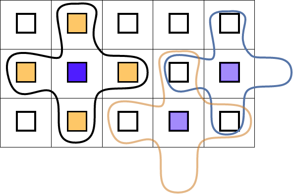
FIGURE 3.9: Illustration of five-point stencil gather
The ever-popular five-point stencil evaluation does not look like a collective operation, and indeed, it is usually evaluated with (nonblocking) send/recv operations. However, if we create a subcommunicator on each subdomain that contains precisely that domain and its neighbors, (see figure 3.9 ) we can formulate the communication pattern as a gather on each of these. With ordinary collectives this can not be formulated in a deadlock -free manner, but nonblocking collectives make this feasible.
We will see an even more elegant formulation of this operation in section 11.2 .
3.11.2 Nonblocking barrier
crumb trail: > mpi-collective > Nonblocking collectives > Nonblocking barrier
Probably the most surprising nonblocking collective is the nonblocking barrier MPI_Ibarrier . The way to understand this is to think of a barrier not in terms of temporal synchronization, but state agreement: reaching a barrier is a sign that a process has attained a certain state, and leaving a barrier means that all processes are in the same state. The ordinary barrier is then a blocking wait for agreement, while with a nonblocking barrier:
- Posting the barrier means that a process has reached a certain state; and
- the request being fullfilled means that all processes have reached the barrier.
One scenario would be local refinement , where some processes decide to refine their subdomain, which fact they need to communicate to their neighbors. The problem here is that most processes are not among these neighbors, so they should not post a receive of any type. Instead, any refining process sends to its neighbors, and every process posts a barrier.
// ibarrierprobe.c
if (i_do_send) {
  /*
   * Pick a random process to send to,
   * not yourself.
   */
  int receiver = rand()%nprocs;
  MPI_Ssend(&data,1,MPI_FLOAT,receiver,0,comm);
}
/*
 * Everyone posts the non-blocking barrier
 * and gets a request to test/wait for
 */
MPI_Request barrier_request;
MPI_Ibarrier(comm,&barrier_request);
Now every process alternately probes for messages and tests for completion of the barrier. Probing is done through the nonblocking MPI_Iprobe call, while testing completion of the barrier is done through MPI_Test .
for ( ; ; step++) {
  int barrier_done_flag=0;
  MPI_Test(&barrier_request,&barrier_done_flag,
           MPI_STATUS_IGNORE);
//stop if you're done!
  if (barrier_done_flag) {
    break;
  } else {
// if you're not done with the barrier:
    int flag; MPI_Status status;
    MPI_Iprobe
      ( MPI_ANY_SOURCE,MPI_ANY_TAG,
        comm, &flag, &status );
    if (flag) {
// absorb message!
We can use a nonblocking barrier to good effect, utilizing the idle time that would result from a blocking barrier. In the following code fragment processes test for completion of the barrier, and failing to detect such completion, perform some local work.
// findbarrier.c MPI_Request final_barrier; MPI_Ibarrier(comm,&final_barrier);int global_finish=mysleep; do { int all_done_flag=0; MPI_Test(&final_barrier,&all_done_flag,MPI_STATUS_IGNORE); if (all_done_flag) { break; } else { int flag; MPI_Status status; // force progress MPI_Iprobe ( MPI_ANY_SOURCE,MPI_ANY_TAG, comm, &flag, MPI_STATUS_IGNORE ); printf("[%d] going to work for another second\n",procid); sleep(1); global_finish++; } } while (1);
3.12 Performance of collectives
crumb trail: > mpi-collective > Performance of collectives
It is easy to visualize a broadcast as in figure 3.10 : see figure 3.10 .
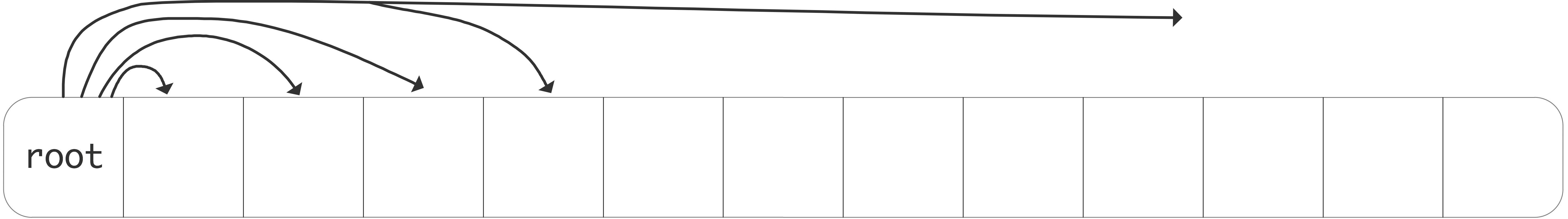
FIGURE 3.10: A simple broadcast
the root sends all of its data directly to every other process. While this describes the semantics of the operation, in practice the implementation works quite differently.
The time that a message takes can simply be modeled as \begin{equation} \alpha +\beta n, \end{equation} where $\alpha$ is the latency , a one time delay from establishing the communication between two processes, and $\beta$ is the time-per-byte, or the inverse of the bandwidth , and $n$ the number of bytes sent.
Under the assumption that a processor can only send one message at a time, the broadcast in figure 3.10 would take a time proportional to the number of processors.
Exercise
What is the total time required for a broadcast involving $p$
processes?
Give $\alpha$ and $\beta$ terms separately.
End of exercise
One way to ameliorate that is to structure the broadcast in a tree-like fashion.
FIGURE 3.11: A tree-based broadcast
This is depicted in figure 3.11 .
Exercise How does the communication time now depend on the number of processors, again $\alpha$ and $\beta$ terms separately.
What would be a lower bound on the $\alpha,\beta$ terms?
End of exercise
The theory of the complexity of collectives is described in more detail in Eijkhout:IntroHPC ; see also [Chan2007Collective] .
3.13 Collectives and synchronization
crumb trail: > mpi-collective > Collectives and synchronization
Collectives, other than a barrier, have a synchronizing effect between processors. For instance, in
MPI_Bcast( ....data... root);
MPI_Send(....);
the send operations on all processors will occur after the root executes the broadcast.
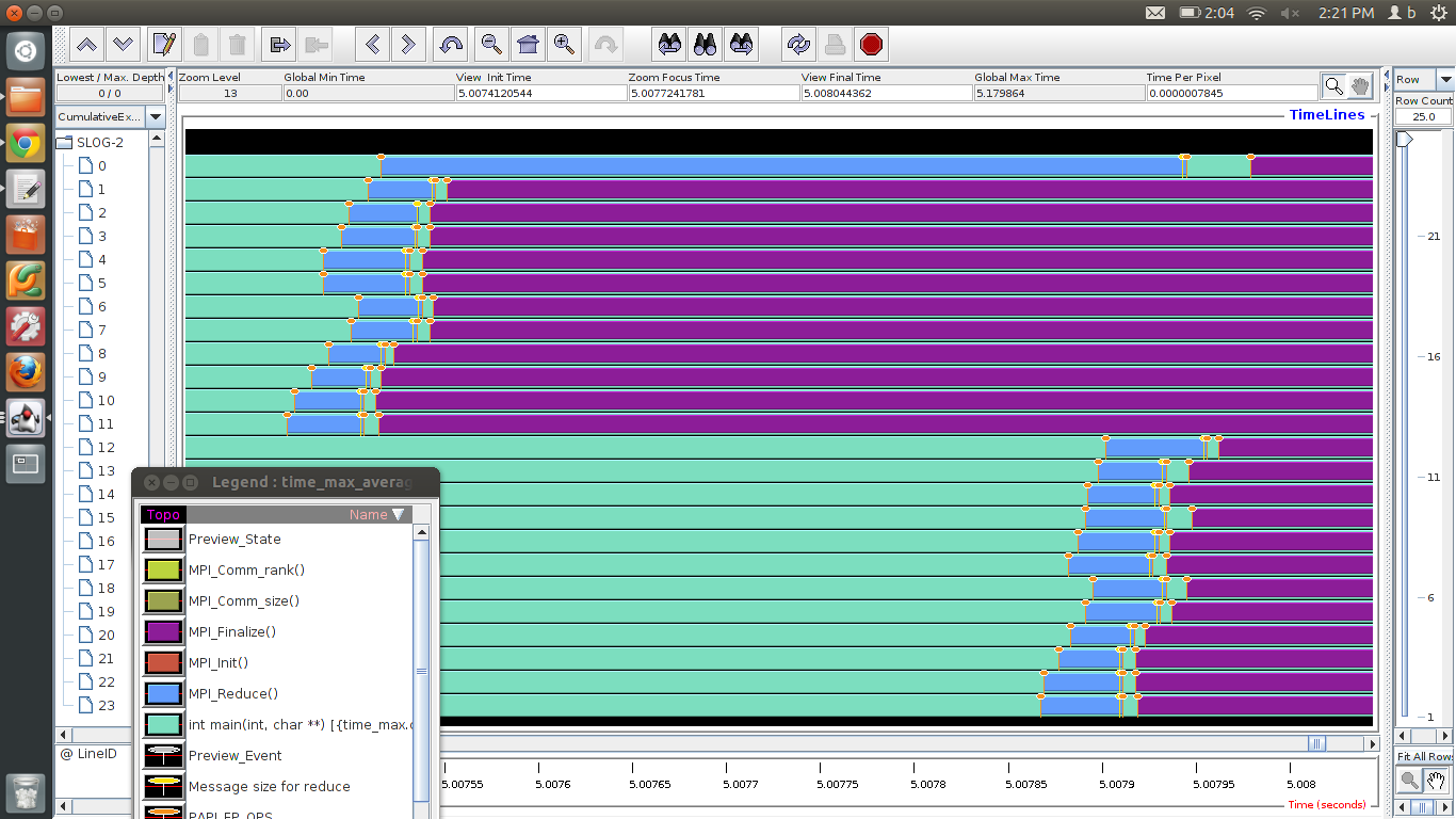
FIGURE 3.12: Trace of a reduction operation between two dual-socket 12-core nodes
Conversely, in a reduce operation the root may have to wait for other processors. This is illustrated in figure 3.12 , which gives a TAU trace of a reduction operation on two nodes, with two six-core sockets (processors) each. We see that\footnote {This uses mvapich version 1.6; in version 1.9 the implementation of an on-node reduction has changed to simulate shared memory.}:
- In each socket, the reduction is a linear accumulation;
- on each node, cores zero and six then combine their result;
- after which the final accumulation is done through the network.
\footnotesize \leftskip=\unitindent \rightskip=\unitindent The most logical execution is:\par\medskip
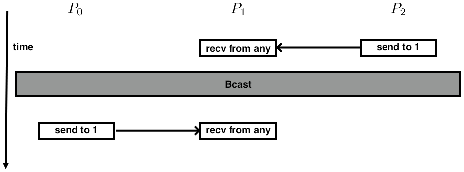
However, this ordering is allowed too:\par\medskip
Which looks from a distance like:\par\medskip
In other words, one of the messages seems to go `back in time'.
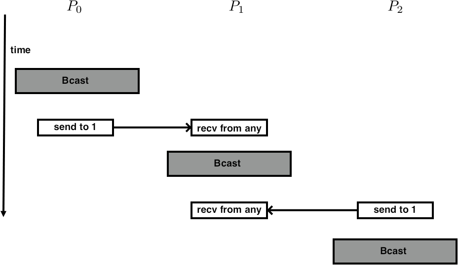
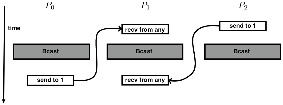
FIGURE 3.13: Possible temporal orderings of send and collective calls
While collectives synchronize in a loose sense, it is not possible to make any statements about events before and after the collectives between processors:
 ...event 1...
MPI_Bcast(....);
 ...event 2....
Consider a specific scenario:
switch(rank) {
    case 0:
        MPI_Bcast(buf1, count, type, 0, comm);
        MPI_Send(buf2, count, type, 1, tag, comm);
        break;
    case 1:
        MPI_Recv(buf2, count, type, MPI_ANY_SOURCE, tag, comm, &status);
        MPI_Bcast(buf1, count, type, 0, comm);
        MPI_Recv(buf2, count, type, MPI_ANY_SOURCE, tag, comm, &status);
        break;
    case 2:
        MPI_Send(buf2, count, type, 1, tag, comm);
        MPI_Bcast(buf1, count, type, 0, comm);
        break;
}
Note the
MPI_ANY_SOURCE
parameter in the receive calls on processor 1.
One obvious execution of this would be:
- The send from 2 is caught by processor 1;
- Everyone executes the broadcast;
- The send from 0 is caught by processor 1.
- Processor 0 starts its broadcast, then executes the send;
- Processor 1's receive catches the data from 0, then it executes its part of the broadcast;
- Processor 1 catches the data sent by 2, and finally processor 2 does its part of the broadcast.
This is illustrated in figure 3.13 .
3.14 Performance considerations
crumb trail: > mpi-collective > Performance considerations
In this section we will consider how collectives can be implemented in multiple ways, and the performance implications of such decisions. You can test the algorithms described here using SimGrid (section \CARPref{tut:simgrid}).
3.14.1 Scalability
crumb trail: > mpi-collective > Performance considerations > Scalability
We are motivated to write parallel software from two considerations. First of all, if we have a certain problem to solve which normally takes time $T$, then we hope that with $p$ processors it will take time $T/p$. If this is true, we call our parallelization scheme scalable in time . In practice, we often accept small extra terms: as you will see below, parallelization often adds a term $\log_2p$ to the running time.
Exercise Discuss scalability of the following algorithms:
- You have an array of floating point numbers. You need to compute the sine of each
- You a two-dimensional array, denoting the interval $[-2,2]^2$. You want to make a picture of the Mandelbrot set , so you need to compute the color of each point.
- The primality test of exercise 2.4 .
End of exercise
There is also the notion that a parallel algorithm can be scalable in space : more processors gives you more memory so that you can run a larger problem.
Exercise
Discuss space scalability in the context of modern processor design.
End of exercise
3.14.2 Complexity and scalability of collectives
crumb trail: > mpi-collective > Performance considerations > Complexity and scalability of collectives
3.14.2.1 Broadcast
crumb trail: > mpi-collective > Performance considerations > Complexity and scalability of collectives > Broadcast
Naive broadcast
Write a broadcast operation where the root does an MPI_Send to each other process.
What is the expected performance of this in terms of $\alpha,\beta$?
Run some tests and confirm.
Simple ring
Let the root only send to the next process, and that one send to its neighbor. This scheme is known as a bucket brigade ; see also section 4.1.5 .
What is the expected performance of this in terms of $\alpha,\beta$?
Run some tests and confirm.
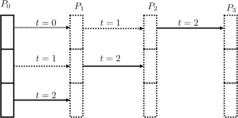
FIGURE 3.14: A pipelined bucket brigade
Pipelined ring
In a ring broadcast, each process needs to receive the whole message before it can pass it on. We can increase the efficiency by breaking up the message and sending it in multiple parts. (See figure 3.14 .) This will be advantageous for messages that are long enough that the bandwidth cost dominates the latency.
Assume a send buffer of length more than 1. Divide the send buffer into a number of chunks. The root sends the chunks successively to the next process, and each process sends on whatever chunks it receives.
What is the expected performance of this in terms of $\alpha,\beta$? Why is this better than the simple ring?
Run some tests and confirm.
Recursive doubling
Collectives such as broadcast can be implemented through recursive doubling , where the root sends to another process, then the root and the other process send to two more, those four send to four more, et cetera. However, in an actual physical architecture this scheme can be realized in multiple ways that have drastically different performance.
First consider the implementation where process 0 is the root, and it starts by sending to process 1; then they send to 2 and 3; these four send to 4--7, et cetera. If the architecture is a linear array of procesors, this will lead to contention : multiple messages wanting to go through the same wire. (This is also related to the concept of bisecection bandwidth .)
In the following analyses we will assume wormhole routing : a message sets up a path through the network, reserving the necessary wires, and performing a send in time independent of the distance through the network. That is, the send time for any message can be modeled as \begin{equation} T(n)=\alpha+\beta n \end{equation} regardless source and destination, as long as the necessary connections are available.
Exercise Analyze the running time of a recursive doubling broad cast as just described, with wormhole routing.
Implement this broadcast in terms of blocking MPI send and receive calls.
If you have SimGrid available, run
tests with a number of parameters.
End of exercise
The alternative, that avoids contention, is to let each doubling stage divide the network into separate halves. That is, process 0 sends to $P/2$, after which these two repeat the algorithm in the two halves of the network, sending to $P/4$ and $3P/4$ respectively.
Exercise
Analyze this variant of recursive doubling. Code it and measure
runtimes on SimGrid.
End of exercise
Exercise Revisit exercise 3.14 and replace the blocking calls by nonblocking MPI_Isend / MPI_Irecv calls.
Make sure to test that the data is correctly propagated.
End of exercise
MPI implementations often have multiple algorithms, which they dynamicaly switch between. Sometimes you can determine the choice yourself through environment variables.
TACC note For Intel MPI , see
3.15 Review questions
crumb trail: > mpi-collective > Review questions
For all true/false questions, if you answer that a statement is false, give a one-line explanation.
Review How would you realize the following scenarios with MPI collectives?
- Let each process compute a random number. You want to print the maximum of these numbers to your screen.
- Each process computes a random number again. Now you want to scale these numbers by their maximum.
- Let each process compute a random number. You want to print on what processor the maximum value is computed.
End of review
Review MPI collectives can be sorted in at least the following categories
- rooted vs rootless
- using uniform buffer lengths vs variable length buffers
- blocking vs nonblocking.
End of review
Review
True or false: collective routines are all about
communicating user data between the processes.
End of review
Review
True or false: an
MPI_Scatter
call puts the same data on
each process.
End of review
Review
True or false: using the option
MPI_IN_PLACE
you
only need space for a send buffer in
MPI_Reduce
.
End of review
Review
True or false: using the option
MPI_IN_PLACE
you
only need space for a send buffer in
MPI_Gather
.
End of review
Review Given a distributed array, with every processor storing
double x[N]; // N can vary per processorgive the approximate MPI-based code that computes the maximum value in the array, and leaves the result on every processor.
End of review
Review
double data[Nglobal];
int myfirst = /* something */, mylast = /* something */;
for (int i=myfirst; i<mylast; i++) {
  if (i>0 && i<N-1) {
    process_point( data,i,Nglobal );
  }
}
void process_point( double *data,int i,int N ) {
    data[i-1] = g(i-1); data[i] = g(i); data[i+1] = g(i+1);
    data[i] = f(data[i-1],data[i],data[i+1]);
}
Is this scalable in time? Is this scalable in space?
What is the missing MPI call?
End of review
Review
double data[Nlocal+2]; // include left and right neighbor
int myfirst = /* something */, mylast = myfirst+Nlocal;
for (int i=0; i<Nlocal; i++) {
  if (i>0 && i<N-1) {
    process_point( data,i,Nlocal );
}
void process_point( double *data,int i0,int n ) {
  int i = i0+1;
  data[i-1] = g(i-1); data[i] = g(i); data[i+1] = g(i+1);
  data[i] = f(data[i-1],data[i],data[i+1]);
}
Is this scalable in time? Is this scalable in space?
What is the missing MPI call?
End of review
Review
With data as in the previous question, given the code for
normalizing the array, that is, scaling each element so that $\|x\|_2=1$.
End of review
Review Just like MPI_Allreduce is equivalent to MPI_Reduce following by MPI_Bcast , MPI_Reduce_scatter is equivalent to at least one of the following combinations. Select those that are equivalent, and discuss differences in time or space complexity:
- MPI_Reduce followed by MPI_Scatter ;
- MPI_Gather followed by MPI_Scatter ;
- MPI_Allreduce followed by MPI_Scatter ;
- MPI_Allreduce followed by a local operation (which?);
- MPI_Allgather followed by a local operation (which?).
End of review
Review
Think of at least two algorithms for doing a broadcast.
Compare them with regards to asymptotic behavior.
End of review